
Applications of Linear Systems
Applications of linear systems turn real problems into equations and solve them by row reduction. To balance a chemical equation, write one equation per element so atoms are conserved. To analyze network flow, write one equation per junction so flow in equals flow out. Free variables then describe every possible answer.
Before this lesson: Gaussian Elimination and Reduced Row Echelon Form
From a word problem to a linear system
Many problems in science and engineering come down to a conservation law: something is neither created nor destroyed. Atoms are conserved in a chemical reaction, and cars or water are conserved at a junction. Each conservation law gives one linear equation.
Once you have the equations, the work is the same as in Gaussian elimination: write the matrix, row reduce and read the solution. The new part is the last step. The answer must make sense in the problem, so coefficients in chemistry must be positive whole numbers and one-way flows can’t be negative.
How to solve applications of linear systems
- Name the unknowns: one variable for each coefficient or each unknown flow.
- Write one linear equation for each conservation law (each element, or each junction).
- Move every variable term to the left side and write the augmented matrix. For a homogeneous system (all constants 0), the coefficient matrix is enough, because a zero column never changes.
- Row reduce to echelon form or to RREF.
- Write the general solution with a free variable t.
- Apply the problem’s limits: whole numbers, positive coefficients or flows of at least 0.
Balancing chemical equations with linear algebra
Put an unknown coefficient in front of every substance, for example x_1\,\text{C}_3\text{H}_8 + x_2\,\text{O}_2 \to x_3\,\text{CO}_2 + x_4\,\text{H}_2\text{O}. For each element, count its atoms on the left and on the right and set the counts equal.
\text{atoms of an element on the left} = \text{atoms of that element on the right}The system is homogeneous (every constant is 0), so it always has the zero solution x₁ = x₂ = … = 0, which is useless here. A balanced equation exists because the system has a free variable. Every solution is a multiple of one vector, and we choose the multiple that makes all coefficients the smallest positive whole numbers. That multiple is the least common multiple of the denominators.
Network flow
A network is a set of junctions (nodes) joined by branches, such as streets, pipes or wires. Each branch carries a flow in a set direction. At every node the flow is conserved.
\text{flow into a node} = \text{flow out of the node}The total flow into the whole network must also equal the total flow out. If it doesn’t, the system is inconsistent. A network usually has a free variable, so there are many possible flows, and limits such as x ≥ 0 on one-way streets narrow them down to a range.
Applications of linear systems examples
Example 1: Balance the combustion of propane
Balance x_1\,\text{C}_3\text{H}_8 + x_2\,\text{O}_2 \to x_3\,\text{CO}_2 + x_4\,\text{H}_2\text{O}.
3x_1 - x_3 = 0
Carbon: 3 atoms in C₃H₈ on the left, 1 in CO₂ on the right, so 3x₁ = x₃.
8x_1 - 2x_4 = 0
Hydrogen: 8 in C₃H₈, 2 in H₂O, so 8x₁ = 2x₄.
2x_2 - 2x_3 - x_4 = 0
Oxygen: 2 in O₂ on the left; 2 in CO₂ and 1 in H₂O on the right.
\begin{bmatrix} 3 & 0 & -1 & 0 \\ 8 & 0 & 0 & -2 \\ 0 & 2 & -2 & -1 \end{bmatrix}Coefficient matrix (columns x₁, x₂, x₃, x₄).
\begin{bmatrix} 3 & 0 & -1 & 0 \\ 0 & 2 & -2 & -1 \\ 8 & 0 & 0 & -2 \end{bmatrix}R₂ ↔ R₃.
\begin{bmatrix} 3 & 0 & -1 & 0 \\ 0 & 2 & -2 & -1 \\ 0 & 0 & \tfrac{8}{3} & -2 \end{bmatrix}R₃ − (8/3)R₁ → R₃.
\begin{bmatrix} 3 & 0 & -1 & 0 \\ 0 & 2 & -2 & -1 \\ 0 & 0 & 1 & -\tfrac{3}{4} \end{bmatrix}(3/8)R₃ → R₃.
\begin{bmatrix} 3 & 0 & -1 & 0 \\ 0 & 2 & 0 & -\tfrac{5}{2} \\ 0 & 0 & 1 & -\tfrac{3}{4} \end{bmatrix}R₂ + 2R₃ → R₂.
\begin{bmatrix} 3 & 0 & -1 & 0 \\ 0 & 1 & 0 & -\tfrac{5}{4} \\ 0 & 0 & 1 & -\tfrac{3}{4} \end{bmatrix}(1/2)R₂ → R₂.
\begin{bmatrix} 3 & 0 & 0 & -\tfrac{3}{4} \\ 0 & 1 & 0 & -\tfrac{5}{4} \\ 0 & 0 & 1 & -\tfrac{3}{4} \end{bmatrix}R₁ + R₃ → R₁.
\begin{bmatrix} 1 & 0 & 0 & -\tfrac{1}{4} \\ 0 & 1 & 0 & -\tfrac{5}{4} \\ 0 & 0 & 1 & -\tfrac{3}{4} \end{bmatrix}(1/3)R₁ → R₁. This is RREF; x₄ is free.
x_1 = \tfrac{1}{4}tLet x₄ = t. Row 1 says x₁ − (1/4)x₄ = 0.
x_2 = \tfrac{5}{4}tRow 2 says x₂ − (5/4)x₄ = 0.
x_3 = \tfrac{3}{4}tRow 3 says x₃ − (3/4)x₄ = 0.
(x_1, x_2, x_3, x_4) = (1, 5, 3, 4)
Choose t = 4, the least common multiple of the denominators.
Answer: \text{C}_3\text{H}_8 + 5\,\text{O}_2 \to 3\,\text{CO}_2 + 4\,\text{H}_2\text{O}. Check: C 3 = 3, H 8 = 8, O 10 = 6 + 4.
Example 2: Fractions in the solution
Balance x_1\,\text{NH}_3 + x_2\,\text{O}_2 \to x_3\,\text{NO} + x_4\,\text{H}_2\text{O}.
x_1 - x_3 = 0
Nitrogen: 1 in NH₃, 1 in NO.
3x_1 - 2x_4 = 0
Hydrogen: 3 in NH₃, 2 in H₂O.
2x_2 - x_3 - x_4 = 0
Oxygen: 2 in O₂; 1 in NO and 1 in H₂O.
\begin{bmatrix} 1 & 0 & -1 & 0 \\ 3 & 0 & 0 & -2 \\ 0 & 2 & -1 & -1 \end{bmatrix}Coefficient matrix.
\begin{bmatrix} 1 & 0 & -1 & 0 \\ 0 & 0 & 3 & -2 \\ 0 & 2 & -1 & -1 \end{bmatrix}R₂ − 3R₁ → R₂.
\begin{bmatrix} 1 & 0 & -1 & 0 \\ 0 & 2 & -1 & -1 \\ 0 & 0 & 3 & -2 \end{bmatrix}R₂ ↔ R₃. Now the pivots step down to the right.
\begin{bmatrix} 1 & 0 & -1 & 0 \\ 0 & 2 & -1 & -1 \\ 0 & 0 & 1 & -\tfrac{2}{3} \end{bmatrix}(1/3)R₃ → R₃.
\begin{bmatrix} 1 & 0 & -1 & 0 \\ 0 & 2 & 0 & -\tfrac{5}{3} \\ 0 & 0 & 1 & -\tfrac{2}{3} \end{bmatrix}R₂ + R₃ → R₂.
\begin{bmatrix} 1 & 0 & -1 & 0 \\ 0 & 1 & 0 & -\tfrac{5}{6} \\ 0 & 0 & 1 & -\tfrac{2}{3} \end{bmatrix}(1/2)R₂ → R₂.
\begin{bmatrix} 1 & 0 & 0 & -\tfrac{2}{3} \\ 0 & 1 & 0 & -\tfrac{5}{6} \\ 0 & 0 & 1 & -\tfrac{2}{3} \end{bmatrix}R₁ + R₃ → R₁. This is RREF.
x_1 = \tfrac{2}{3}t,\; x_2 = \tfrac{5}{6}t,\; x_3 = \tfrac{2}{3}t,\; x_4 = tLet x₄ = t and read each row.
(x_1, x_2, x_3, x_4) = (4, 5, 4, 6)
The denominators are 3, 6 and 3; their least common multiple is 6, so t = 6.
Answer: 4\,\text{NH}_3 + 5\,\text{O}_2 \to 4\,\text{NO} + 6\,\text{H}_2\text{O}. Check: N 4 = 4, H 12 = 12, O 10 = 4 + 6.
Example 3: Six unknowns
Balance x_1\,\text{KMnO}_4 + x_2\,\text{HCl} \to x_3\,\text{KCl} + x_4\,\text{MnCl}_2 + x_5\,\text{H}_2\text{O} + x_6\,\text{Cl}_2.
x_1 - x_3 = 0
Potassium (K): 1 in KMnO₄, 1 in KCl.
x_2 - 2x_5 = 0
Hydrogen: 1 in HCl, 2 in H₂O.
x_1 - x_4 = 0
Manganese (Mn): 1 in KMnO₄, 1 in MnCl₂.
4x_1 - x_5 = 0
Oxygen: 4 in KMnO₄, 1 in H₂O.
x_2 - x_3 - 2x_4 - 2x_6 = 0
Chlorine: 1 in HCl; 1 in KCl, 2 in MnCl₂ and 2 in Cl₂.
\begin{bmatrix} 1 & 0 & -1 & 0 & 0 & 0 \\ 0 & 1 & 0 & 0 & -2 & 0 \\ 1 & 0 & 0 & -1 & 0 & 0 \\ 4 & 0 & 0 & 0 & -1 & 0 \\ 0 & 1 & -1 & -2 & 0 & -2 \end{bmatrix}Coefficient matrix, rows in the order K, H, Mn, O, Cl.
\begin{bmatrix} 1 & 0 & -1 & 0 & 0 & 0 \\ 0 & 1 & 0 & 0 & -2 & 0 \\ 0 & 0 & 1 & -1 & 0 & 0 \\ 4 & 0 & 0 & 0 & -1 & 0 \\ 0 & 1 & -1 & -2 & 0 & -2 \end{bmatrix}R₃ − R₁ → R₃.
\begin{bmatrix} 1 & 0 & -1 & 0 & 0 & 0 \\ 0 & 1 & 0 & 0 & -2 & 0 \\ 0 & 0 & 1 & -1 & 0 & 0 \\ 0 & 0 & 4 & 0 & -1 & 0 \\ 0 & 1 & -1 & -2 & 0 & -2 \end{bmatrix}R₄ − 4R₁ → R₄.
\begin{bmatrix} 1 & 0 & -1 & 0 & 0 & 0 \\ 0 & 1 & 0 & 0 & -2 & 0 \\ 0 & 0 & 1 & -1 & 0 & 0 \\ 0 & 0 & 4 & 0 & -1 & 0 \\ 0 & 0 & -1 & -2 & 2 & -2 \end{bmatrix}R₅ − R₂ → R₅.
\begin{bmatrix} 1 & 0 & -1 & 0 & 0 & 0 \\ 0 & 1 & 0 & 0 & -2 & 0 \\ 0 & 0 & 1 & -1 & 0 & 0 \\ 0 & 0 & 0 & 4 & -1 & 0 \\ 0 & 0 & -1 & -2 & 2 & -2 \end{bmatrix}R₄ − 4R₃ → R₄.
\begin{bmatrix} 1 & 0 & -1 & 0 & 0 & 0 \\ 0 & 1 & 0 & 0 & -2 & 0 \\ 0 & 0 & 1 & -1 & 0 & 0 \\ 0 & 0 & 0 & 4 & -1 & 0 \\ 0 & 0 & 0 & -3 & 2 & -2 \end{bmatrix}R₅ + R₃ → R₅.
\begin{bmatrix} 1 & 0 & -1 & 0 & 0 & 0 \\ 0 & 1 & 0 & 0 & -2 & 0 \\ 0 & 0 & 1 & -1 & 0 & 0 \\ 0 & 0 & 0 & 1 & -\tfrac{1}{4} & 0 \\ 0 & 0 & 0 & -3 & 2 & -2 \end{bmatrix}(1/4)R₄ → R₄.
\begin{bmatrix} 1 & 0 & -1 & 0 & 0 & 0 \\ 0 & 1 & 0 & 0 & -2 & 0 \\ 0 & 0 & 1 & -1 & 0 & 0 \\ 0 & 0 & 0 & 1 & -\tfrac{1}{4} & 0 \\ 0 & 0 & 0 & 0 & \tfrac{5}{4} & -2 \end{bmatrix}R₅ + 3R₄ → R₅.
\begin{bmatrix} 1 & 0 & -1 & 0 & 0 & 0 \\ 0 & 1 & 0 & 0 & -2 & 0 \\ 0 & 0 & 1 & -1 & 0 & 0 \\ 0 & 0 & 0 & 1 & -\tfrac{1}{4} & 0 \\ 0 & 0 & 0 & 0 & 1 & -\tfrac{8}{5} \end{bmatrix}(4/5)R₅ → R₅. Echelon form; x₆ is free.
x_5 = \tfrac{8}{5}tLet x₆ = t. Row 5: x₅ − (8/5)x₆ = 0.
x_4 = \tfrac{1}{4}x_5 = \tfrac{2}{5}tRow 4: x₄ − (1/4)x₅ = 0; back substitute.
x_3 = x_4 = \tfrac{2}{5}tRow 3: x₃ − x₄ = 0.
x_2 = 2x_5 = \tfrac{16}{5}tRow 2: x₂ − 2x₅ = 0.
x_1 = x_3 = \tfrac{2}{5}tRow 1: x₁ − x₃ = 0.
(x_1, \dots, x_6) = (2, 16, 2, 2, 8, 5)
Every denominator is 5, so t = 5.
Answer: 2\,\text{KMnO}_4 + 16\,\text{HCl} \to 2\,\text{KCl} + 2\,\text{MnCl}_2 + 8\,\text{H}_2\text{O} + 5\,\text{Cl}_2. Check: Cl 16 = 2 + 4 + 10, O 8 = 8, H 16 = 16.
Example 4: Flow in a pipe network
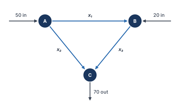
Water enters junction A at 50 L/min and junction B at 20 L/min, and leaves junction C at 70 L/min. Pipes carry x₁ from A to B, x₂ from A to C and x₃ from B to C. Find every possible flow.
x_1 + x_2 = 50
Junction A: 50 in; x₁ and x₂ out.
x_1 - x_3 = -20
Junction B: x₁ + 20 in; x₃ out. Subtract x₃ and 20 from both sides.
x_2 + x_3 = 70
Junction C: x₂ + x₃ in; 70 out.
\left[\begin{array}{rrr|r} 1 & 1 & 0 & 50 \\ 1 & 0 & -1 & -20 \\ 0 & 1 & 1 & 70 \end{array}\right]Augmented matrix.
\left[\begin{array}{rrr|r} 1 & 1 & 0 & 50 \\ 0 & -1 & -1 & -70 \\ 0 & 1 & 1 & 70 \end{array}\right]R₂ − R₁ → R₂.
\left[\begin{array}{rrr|r} 1 & 1 & 0 & 50 \\ 0 & 1 & 1 & 70 \\ 0 & 1 & 1 & 70 \end{array}\right]−R₂ → R₂.
\left[\begin{array}{rrr|r} 1 & 1 & 0 & 50 \\ 0 & 1 & 1 & 70 \\ 0 & 0 & 0 & 0 \end{array}\right]R₃ − R₂ → R₃. One equation was redundant: total in, 70, equals total out.
\left[\begin{array}{rrr|r} 1 & 0 & -1 & -20 \\ 0 & 1 & 1 & 70 \\ 0 & 0 & 0 & 0 \end{array}\right]R₁ − R₂ → R₁. This is RREF; x₃ is free.
x_1 = -20 + t,\; x_2 = 70 - t,\; x_3 = t
Let x₃ = t and solve each row.
20 \le t \le 70
Each flow must be at least 0: x₁ ≥ 0 gives t ≥ 20 and x₂ ≥ 0 gives t ≤ 70.
Answer: x₁ = t − 20, x₂ = 70 − t, x₃ = t, with 20 ≤ t ≤ 70. For example, t = 40 gives flows of 20, 30 and 40 L/min.
Example 5: Traffic around a city block
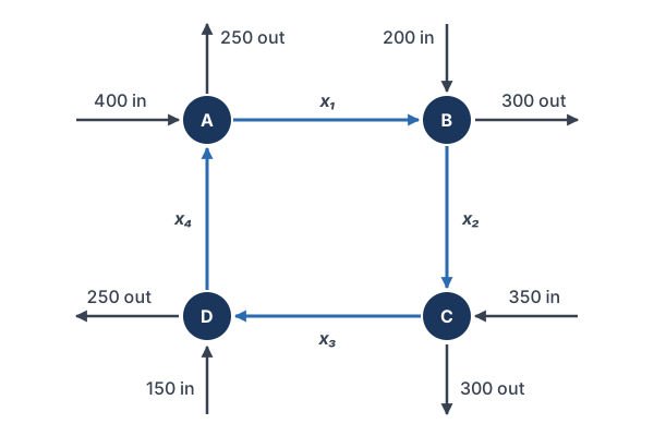
Four one-way streets form a loop around a block, with traffic counted in cars per hour. At A, 400 cars enter and 250 leave; at B, 200 enter and 300 leave; at C, 350 enter and 300 leave; at D, 150 enter and 250 leave. Inside the loop, x₁ runs A to B, x₂ runs B to C, x₃ runs C to D and x₄ runs D to A. (a) Find the general flow. (b) If street DA is closed for repairs, what are the other flows? (c) What is the smallest possible flow on AB?
x_1 - x_4 = 150
A: x₄ + 400 in = x₁ + 250 out; move terms.
x_1 - x_2 = 100
B: x₁ + 200 = x₂ + 300.
x_2 - x_3 = -50
C: x₂ + 350 = x₃ + 300.
x_3 - x_4 = 100
D: x₃ + 150 = x₄ + 250.
\left[\begin{array}{rrrr|r} 1 & 0 & 0 & -1 & 150 \\ 1 & -1 & 0 & 0 & 100 \\ 0 & 1 & -1 & 0 & -50 \\ 0 & 0 & 1 & -1 & 100 \end{array}\right]Augmented matrix.
\left[\begin{array}{rrrr|r} 1 & 0 & 0 & -1 & 150 \\ 0 & -1 & 0 & 1 & -50 \\ 0 & 1 & -1 & 0 & -50 \\ 0 & 0 & 1 & -1 & 100 \end{array}\right]R₂ − R₁ → R₂.
\left[\begin{array}{rrrr|r} 1 & 0 & 0 & -1 & 150 \\ 0 & 1 & 0 & -1 & 50 \\ 0 & 1 & -1 & 0 & -50 \\ 0 & 0 & 1 & -1 & 100 \end{array}\right]−R₂ → R₂.
\left[\begin{array}{rrrr|r} 1 & 0 & 0 & -1 & 150 \\ 0 & 1 & 0 & -1 & 50 \\ 0 & 0 & -1 & 1 & -100 \\ 0 & 0 & 1 & -1 & 100 \end{array}\right]R₃ − R₂ → R₃.
\left[\begin{array}{rrrr|r} 1 & 0 & 0 & -1 & 150 \\ 0 & 1 & 0 & -1 & 50 \\ 0 & 0 & 1 & -1 & 100 \\ 0 & 0 & 1 & -1 & 100 \end{array}\right]−R₃ → R₃.
\left[\begin{array}{rrrr|r} 1 & 0 & 0 & -1 & 150 \\ 0 & 1 & 0 & -1 & 50 \\ 0 & 0 & 1 & -1 & 100 \\ 0 & 0 & 0 & 0 & 0 \end{array}\right]R₄ − R₃ → R₄. This is RREF; x₄ is free.
x_1 = 150 + t,\; x_2 = 50 + t,\; x_3 = 100 + t,\; x_4 = t
(a) Let x₄ = t ≥ 0.
(x_1, x_2, x_3) = (150, 50, 100)
(b) Closing DA means t = 0.
x_1 = 150 + t \ge 150
(c) The least value of t is 0.
Answer: (a) (x₁, x₂, x₃, x₄) = (150 + t, 50 + t, 100 + t, t) for t ≥ 0. (b) 150, 50 and 100 cars per hour. (c) At least 150 cars per hour must use AB.
Common mistakes
| Mistake | Example of the error | Fix |
|---|---|---|
| Leaving product terms on the right | Writing 3x₁ + x₃ = 0 for carbon in Example 1 | Atoms on the right are subtracted: 3x₁ − x₃ = 0. |
| Miscounting atoms in a group | Counting 3 oxygen atoms in Cu(NO₃)₂ | Multiply through the parentheses: 2 × 3 = 6 oxygen atoms. |
| Stopping at fractions | Answering (1/4, 5/4, 3/4, 1) in Example 1 | Multiply by the least common multiple of the denominators to get whole numbers. |
| Giving a non-smallest answer | (2, 10, 6, 8) for propane | It balances, but divide by the common factor 2 for the standard answer. |
| Dropping outside flows | Writing x₁ = x₄ at node A in Example 5 | Include the 400 entering and the 250 leaving. |
| Ignoring direction limits | Allowing t = 0 in Example 4, which makes x₁ = −20 | One-way flows must be at least 0, so 20 ≤ t ≤ 70. |
Related methods
Balancing by inspection
For short equations, chemists often balance by trial: fix one coefficient, then adjust the others element by element. The matrix method gives the same answer, and it is better for long equations like Example 3, where trial and error gets lost.
Polynomial curve fitting
To find the polynomial y = a + bx + cx² through three points, substitute each point to get three linear equations in a, b and c. This is the same idea as systems of equations in three variables, and Practice Problem 10 does one with row reduction.
Electrical circuits
Kirchhoff’s current law says the current into each junction equals the current out, so it is network flow. Kirchhoff’s voltage law adds one equation per loop, and the currents come from the same row reduction.
Practice problems
- Balance x_1\,\text{H}_2\text{O}_2 \to x_2\,\text{H}_2\text{O} + x_3\,\text{O}_2.
- Balance x_1\,\text{CH}_4 + x_2\,\text{O}_2 \to x_3\,\text{CO}_2 + x_4\,\text{H}_2\text{O}.
- Balance x_1\,\text{Al} + x_2\,\text{O}_2 \to x_3\,\text{Al}_2\text{O}_3.
- Balance x_1\,\text{C}_2\text{H}_6 + x_2\,\text{O}_2 \to x_3\,\text{CO}_2 + x_4\,\text{H}_2\text{O}.
- Balance x_1\,\text{Fe}_2\text{O}_3 + x_2\,\text{CO} \to x_3\,\text{Fe} + x_4\,\text{CO}_2.
- Balance x_1\,\text{C}_3\text{H}_8\text{O} + x_2\,\text{O}_2 \to x_3\,\text{CO}_2 + x_4\,\text{H}_2\text{O}.
- Balance x_1\,\text{Cu} + x_2\,\text{HNO}_3 \to x_3\,\text{Cu(NO}_3\text{)}_2 + x_4\,\text{NO} + x_5\,\text{H}_2\text{O}.
- Water enters junction A at 80 L/min and leaves junction B at 30 L/min and junction C at 50 L/min. Pipes carry x₁ from A to B, x₂ from B to C and x₃ from A to C. Find every possible flow and the smallest possible x₁.
- One-way streets carry x₁ from A to B, x₂ from B to C, x₃ from C to D and x₄ from A to D. At A, 500 cars per hour enter; at B, 200 leave; at C, 100 enter; at D, 400 leave. Find the general flow, the flows if street AD is closed, and the largest possible x₄.
- Find the parabola y = a + bx + cx² through (1, 4), (2, 9) and (3, 18).
Show answers
1.
2x_1 - 2x_2 = 0
Hydrogen: 2 in H₂O₂, 2 in H₂O.
2x_1 - x_2 - 2x_3 = 0
Oxygen: 2 in H₂O₂; 1 in H₂O and 2 in O₂.
\begin{bmatrix} 2 & -2 & 0 \\ 2 & -1 & -2 \end{bmatrix}Coefficient matrix.
\begin{bmatrix} 2 & -2 & 0 \\ 0 & 1 & -2 \end{bmatrix}R₂ − R₁ → R₂.
\begin{bmatrix} 1 & -1 & 0 \\ 0 & 1 & -2 \end{bmatrix}(1/2)R₁ → R₁.
\begin{bmatrix} 1 & 0 & -2 \\ 0 & 1 & -2 \end{bmatrix}R₁ + R₂ → R₁.
x_1 = 2t,\; x_2 = 2t,\; x_3 = t
Let x₃ = t and read each row.
(x_1, x_2, x_3) = (2, 2, 1)
t = 1 already gives whole numbers.
Answer: 2 H₂O₂ → 2 H₂O + O₂
2.
x_1 - x_3 = 0
Carbon.
4x_1 - 2x_4 = 0
Hydrogen.
2x_2 - 2x_3 - x_4 = 0
Oxygen.
\begin{bmatrix} 1 & 0 & -1 & 0 \\ 4 & 0 & 0 & -2 \\ 0 & 2 & -2 & -1 \end{bmatrix}Coefficient matrix.
\begin{bmatrix} 1 & 0 & -1 & 0 \\ 0 & 0 & 4 & -2 \\ 0 & 2 & -2 & -1 \end{bmatrix}R₂ − 4R₁ → R₂.
\begin{bmatrix} 1 & 0 & -1 & 0 \\ 0 & 2 & -2 & -1 \\ 0 & 0 & 4 & -2 \end{bmatrix}R₂ ↔ R₃.
\begin{bmatrix} 1 & 0 & -1 & 0 \\ 0 & 2 & -2 & -1 \\ 0 & 0 & 1 & -\tfrac{1}{2} \end{bmatrix}(1/4)R₃ → R₃.
\begin{bmatrix} 1 & 0 & -1 & 0 \\ 0 & 2 & 0 & -2 \\ 0 & 0 & 1 & -\tfrac{1}{2} \end{bmatrix}R₂ + 2R₃ → R₂.
\begin{bmatrix} 1 & 0 & -1 & 0 \\ 0 & 1 & 0 & -1 \\ 0 & 0 & 1 & -\tfrac{1}{2} \end{bmatrix}(1/2)R₂ → R₂.
\begin{bmatrix} 1 & 0 & 0 & -\tfrac{1}{2} \\ 0 & 1 & 0 & -1 \\ 0 & 0 & 1 & -\tfrac{1}{2} \end{bmatrix}R₁ + R₃ → R₁.
x_1 = \tfrac{1}{2}t,\; x_2 = t,\; x_3 = \tfrac{1}{2}t,\; x_4 = tLet x₄ = t.
(x_1, x_2, x_3, x_4) = (1, 2, 1, 2)
t = 2.
Answer: CH₄ + 2 O₂ → CO₂ + 2 H₂O
3.
x_1 - 2x_3 = 0
Aluminum: 1 in Al, 2 in Al₂O₃.
2x_2 - 3x_3 = 0
Oxygen: 2 in O₂, 3 in Al₂O₃.
\begin{bmatrix} 1 & 0 & -2 \\ 0 & 2 & -3 \end{bmatrix}Coefficient matrix.
\begin{bmatrix} 1 & 0 & -2 \\ 0 & 1 & -\tfrac{3}{2} \end{bmatrix}(1/2)R₂ → R₂.
x_1 = 2t,\; x_2 = \tfrac{3}{2}t,\; x_3 = tLet x₃ = t.
(x_1, x_2, x_3) = (4, 3, 2)
t = 2.
Answer: 4 Al + 3 O₂ → 2 Al₂O₃
4.
2x_1 - x_3 = 0
Carbon.
6x_1 - 2x_4 = 0
Hydrogen.
2x_2 - 2x_3 - x_4 = 0
Oxygen.
\begin{bmatrix} 2 & 0 & -1 & 0 \\ 6 & 0 & 0 & -2 \\ 0 & 2 & -2 & -1 \end{bmatrix}Coefficient matrix.
\begin{bmatrix} 2 & 0 & -1 & 0 \\ 0 & 0 & 3 & -2 \\ 0 & 2 & -2 & -1 \end{bmatrix}R₂ − 3R₁ → R₂.
\begin{bmatrix} 2 & 0 & -1 & 0 \\ 0 & 2 & -2 & -1 \\ 0 & 0 & 3 & -2 \end{bmatrix}R₂ ↔ R₃.
\begin{bmatrix} 2 & 0 & -1 & 0 \\ 0 & 2 & -2 & -1 \\ 0 & 0 & 1 & -\tfrac{2}{3} \end{bmatrix}(1/3)R₃ → R₃.
\begin{bmatrix} 2 & 0 & -1 & 0 \\ 0 & 2 & 0 & -\tfrac{7}{3} \\ 0 & 0 & 1 & -\tfrac{2}{3} \end{bmatrix}R₂ + 2R₃ → R₂.
\begin{bmatrix} 2 & 0 & -1 & 0 \\ 0 & 1 & 0 & -\tfrac{7}{6} \\ 0 & 0 & 1 & -\tfrac{2}{3} \end{bmatrix}(1/2)R₂ → R₂.
\begin{bmatrix} 2 & 0 & 0 & -\tfrac{2}{3} \\ 0 & 1 & 0 & -\tfrac{7}{6} \\ 0 & 0 & 1 & -\tfrac{2}{3} \end{bmatrix}R₁ + R₃ → R₁.
\begin{bmatrix} 1 & 0 & 0 & -\tfrac{1}{3} \\ 0 & 1 & 0 & -\tfrac{7}{6} \\ 0 & 0 & 1 & -\tfrac{2}{3} \end{bmatrix}(1/2)R₁ → R₁.
x_1 = \tfrac{1}{3}t,\; x_2 = \tfrac{7}{6}t,\; x_3 = \tfrac{2}{3}t,\; x_4 = tLet x₄ = t.
(x_1, x_2, x_3, x_4) = (2, 7, 4, 6)
t = 6, the least common multiple of 3, 6 and 3.
Answer: 2 C₂H₆ + 7 O₂ → 4 CO₂ + 6 H₂O
5.
2x_1 - x_3 = 0
Iron.
3x_1 + x_2 - 2x_4 = 0
Oxygen: 3 in Fe₂O₃ and 1 in CO; 2 in CO₂.
x_2 - x_4 = 0
Carbon.
\begin{bmatrix} 2 & 0 & -1 & 0 \\ 3 & 1 & 0 & -2 \\ 0 & 1 & 0 & -1 \end{bmatrix}Coefficient matrix.
\begin{bmatrix} 1 & 0 & -\tfrac{1}{2} & 0 \\ 3 & 1 & 0 & -2 \\ 0 & 1 & 0 & -1 \end{bmatrix}(1/2)R₁ → R₁.
\begin{bmatrix} 1 & 0 & -\tfrac{1}{2} & 0 \\ 0 & 1 & \tfrac{3}{2} & -2 \\ 0 & 1 & 0 & -1 \end{bmatrix}R₂ − 3R₁ → R₂.
\begin{bmatrix} 1 & 0 & -\tfrac{1}{2} & 0 \\ 0 & 1 & \tfrac{3}{2} & -2 \\ 0 & 0 & -\tfrac{3}{2} & 1 \end{bmatrix}R₃ − R₂ → R₃.
\begin{bmatrix} 1 & 0 & -\tfrac{1}{2} & 0 \\ 0 & 1 & \tfrac{3}{2} & -2 \\ 0 & 0 & 1 & -\tfrac{2}{3} \end{bmatrix}−(2/3)R₃ → R₃.
\begin{bmatrix} 1 & 0 & -\tfrac{1}{2} & 0 \\ 0 & 1 & 0 & -1 \\ 0 & 0 & 1 & -\tfrac{2}{3} \end{bmatrix}R₂ − (3/2)R₃ → R₂.
\begin{bmatrix} 1 & 0 & 0 & -\tfrac{1}{3} \\ 0 & 1 & 0 & -1 \\ 0 & 0 & 1 & -\tfrac{2}{3} \end{bmatrix}R₁ + (1/2)R₃ → R₁.
x_1 = \tfrac{1}{3}t,\; x_2 = t,\; x_3 = \tfrac{2}{3}t,\; x_4 = tLet x₄ = t.
(x_1, x_2, x_3, x_4) = (1, 3, 2, 3)
t = 3.
Answer: Fe₂O₃ + 3 CO → 2 Fe + 3 CO₂
6.
x_1 + 2x_2 - 2x_3 - x_4 = 0
Oxygen: 1 in C₃H₈O and 2 in O₂; 2 in CO₂ and 1 in H₂O.
3x_1 - x_3 = 0
Carbon.
8x_1 - 2x_4 = 0
Hydrogen.
\begin{bmatrix} 1 & 2 & -2 & -1 \\ 3 & 0 & -1 & 0 \\ 8 & 0 & 0 & -2 \end{bmatrix}Coefficient matrix, oxygen row first.
\begin{bmatrix} 1 & 2 & -2 & -1 \\ 0 & -6 & 5 & 3 \\ 8 & 0 & 0 & -2 \end{bmatrix}R₂ − 3R₁ → R₂.
\begin{bmatrix} 1 & 2 & -2 & -1 \\ 0 & -6 & 5 & 3 \\ 0 & -16 & 16 & 6 \end{bmatrix}R₃ − 8R₁ → R₃.
\begin{bmatrix} 1 & 2 & -2 & -1 \\ 0 & 1 & -\tfrac{5}{6} & -\tfrac{1}{2} \\ 0 & -16 & 16 & 6 \end{bmatrix}−(1/6)R₂ → R₂.
\begin{bmatrix} 1 & 2 & -2 & -1 \\ 0 & 1 & -\tfrac{5}{6} & -\tfrac{1}{2} \\ 0 & 0 & \tfrac{8}{3} & -2 \end{bmatrix}R₃ + 16R₂ → R₃.
\begin{bmatrix} 1 & 2 & -2 & -1 \\ 0 & 1 & -\tfrac{5}{6} & -\tfrac{1}{2} \\ 0 & 0 & 1 & -\tfrac{3}{4} \end{bmatrix}(3/8)R₃ → R₃.
x_3 = \tfrac{3}{4}tEchelon form. Let x₄ = t; row 3 gives x₃.
x_2 = \tfrac{5}{6}\cdot\tfrac{3}{4}t + \tfrac{1}{2}t = \tfrac{9}{8}tRow 2: x₂ = (5/6)x₃ + (1/2)x₄.
x_1 = -2\cdot\tfrac{9}{8}t + 2\cdot\tfrac{3}{4}t + t = \tfrac{1}{4}tRow 1: x₁ = −2x₂ + 2x₃ + x₄.
(x_1, x_2, x_3, x_4) = (2, 9, 6, 8)
t = 8.
Answer: 2 C₃H₈O + 9 O₂ → 6 CO₂ + 8 H₂O
7.
x_1 - x_3 = 0
Copper.
x_2 - 2x_5 = 0
Hydrogen.
x_2 - 2x_3 - x_4 = 0
Nitrogen: 2 in Cu(NO₃)₂.
3x_2 - 6x_3 - x_4 - x_5 = 0
Oxygen: 3 in HNO₃; 6 in Cu(NO₃)₂, 1 in NO, 1 in H₂O.
\begin{bmatrix} 1 & 0 & -1 & 0 & 0 \\ 0 & 1 & 0 & 0 & -2 \\ 0 & 1 & -2 & -1 & 0 \\ 0 & 3 & -6 & -1 & -1 \end{bmatrix}Coefficient matrix (columns x₁ to x₅).
\begin{bmatrix} 1 & 0 & -1 & 0 & 0 \\ 0 & 1 & 0 & 0 & -2 \\ 0 & 0 & -2 & -1 & 2 \\ 0 & 3 & -6 & -1 & -1 \end{bmatrix}R₃ − R₂ → R₃.
\begin{bmatrix} 1 & 0 & -1 & 0 & 0 \\ 0 & 1 & 0 & 0 & -2 \\ 0 & 0 & -2 & -1 & 2 \\ 0 & 0 & -6 & -1 & 5 \end{bmatrix}R₄ − 3R₂ → R₄.
\begin{bmatrix} 1 & 0 & -1 & 0 & 0 \\ 0 & 1 & 0 & 0 & -2 \\ 0 & 0 & -2 & -1 & 2 \\ 0 & 0 & 0 & 2 & -1 \end{bmatrix}R₄ − 3R₃ → R₄.
\begin{bmatrix} 1 & 0 & -1 & 0 & 0 \\ 0 & 1 & 0 & 0 & -2 \\ 0 & 0 & 1 & \tfrac{1}{2} & -1 \\ 0 & 0 & 0 & 2 & -1 \end{bmatrix}−(1/2)R₃ → R₃.
\begin{bmatrix} 1 & 0 & -1 & 0 & 0 \\ 0 & 1 & 0 & 0 & -2 \\ 0 & 0 & 1 & \tfrac{1}{2} & -1 \\ 0 & 0 & 0 & 1 & -\tfrac{1}{2} \end{bmatrix}(1/2)R₄ → R₄.
x_4 = \tfrac{1}{2}tEchelon form. Let x₅ = t; row 4 gives x₄.
x_3 = -\tfrac{1}{2}\cdot\tfrac{1}{2}t + t = \tfrac{3}{4}tRow 3: x₃ = −(1/2)x₄ + x₅.
x_2 = 2t
Row 2: x₂ = 2x₅.
x_1 = \tfrac{3}{4}tRow 1: x₁ = x₃.
(x_1, \dots, x_5) = (3, 8, 3, 2, 4)
t = 4.
Answer: 3 Cu + 8 HNO₃ → 3 Cu(NO₃)₂ + 2 NO + 4 H₂O
8.
x_1 + x_3 = 80
Junction A: 80 in; x₁ and x₃ out.
x_1 - x_2 = 30
Junction B: x₁ in; x₂ and 30 out.
x_2 + x_3 = 50
Junction C: x₂ and x₃ in; 50 out.
\left[\begin{array}{rrr|r} 1 & 0 & 1 & 80 \\ 1 & -1 & 0 & 30 \\ 0 & 1 & 1 & 50 \end{array}\right]Augmented matrix.
\left[\begin{array}{rrr|r} 1 & 0 & 1 & 80 \\ 0 & -1 & -1 & -50 \\ 0 & 1 & 1 & 50 \end{array}\right]R₂ − R₁ → R₂.
\left[\begin{array}{rrr|r} 1 & 0 & 1 & 80 \\ 0 & 1 & 1 & 50 \\ 0 & 1 & 1 & 50 \end{array}\right]−R₂ → R₂.
\left[\begin{array}{rrr|r} 1 & 0 & 1 & 80 \\ 0 & 1 & 1 & 50 \\ 0 & 0 & 0 & 0 \end{array}\right]R₃ − R₂ → R₃.
x_1 = 80 - t,\; x_2 = 50 - t,\; x_3 = t
RREF; let x₃ = t.
0 \le t \le 50
x₂ ≥ 0 needs t ≤ 50, and x₃ ≥ 0 needs t ≥ 0.
x_1 = 80 - 50 = 30
x₁ is smallest when t is largest.
Answer: x₁ = 80 − t, x₂ = 50 − t, x₃ = t for 0 ≤ t ≤ 50; the smallest x₁ is 30 L/min.
9.
x_1 + x_4 = 500
A: 500 in; x₁ and x₄ out.
x_1 - x_2 = 200
B: x₁ in; x₂ and 200 out.
x_2 - x_3 = -100
C: x₂ + 100 in; x₃ out.
x_3 + x_4 = 400
D: x₃ + x₄ in; 400 out.
\left[\begin{array}{rrrr|r} 1 & 0 & 0 & 1 & 500 \\ 1 & -1 & 0 & 0 & 200 \\ 0 & 1 & -1 & 0 & -100 \\ 0 & 0 & 1 & 1 & 400 \end{array}\right]Augmented matrix.
\left[\begin{array}{rrrr|r} 1 & 0 & 0 & 1 & 500 \\ 0 & -1 & 0 & -1 & -300 \\ 0 & 1 & -1 & 0 & -100 \\ 0 & 0 & 1 & 1 & 400 \end{array}\right]R₂ − R₁ → R₂.
\left[\begin{array}{rrrr|r} 1 & 0 & 0 & 1 & 500 \\ 0 & 1 & 0 & 1 & 300 \\ 0 & 1 & -1 & 0 & -100 \\ 0 & 0 & 1 & 1 & 400 \end{array}\right]−R₂ → R₂.
\left[\begin{array}{rrrr|r} 1 & 0 & 0 & 1 & 500 \\ 0 & 1 & 0 & 1 & 300 \\ 0 & 0 & -1 & -1 & -400 \\ 0 & 0 & 1 & 1 & 400 \end{array}\right]R₃ − R₂ → R₃.
\left[\begin{array}{rrrr|r} 1 & 0 & 0 & 1 & 500 \\ 0 & 1 & 0 & 1 & 300 \\ 0 & 0 & 1 & 1 & 400 \\ 0 & 0 & 1 & 1 & 400 \end{array}\right]−R₃ → R₃.
\left[\begin{array}{rrrr|r} 1 & 0 & 0 & 1 & 500 \\ 0 & 1 & 0 & 1 & 300 \\ 0 & 0 & 1 & 1 & 400 \\ 0 & 0 & 0 & 0 & 0 \end{array}\right]R₄ − R₃ → R₄.
x_1 = 500 - t,\; x_2 = 300 - t,\; x_3 = 400 - t,\; x_4 = t
RREF; let x₄ = t.
(x_1, x_2, x_3) = (500, 300, 400)
Closing AD means t = 0.
0 \le t \le 300
x₂ ≥ 0 needs t ≤ 300, the tightest limit.
Answer: (500 − t, 300 − t, 400 − t, t) for 0 ≤ t ≤ 300; with AD closed the flows are 500, 300 and 400 cars per hour; the largest x₄ is 300.
10.
a + b + c = 4
Substitute (1, 4).
a + 2b + 4c = 9
Substitute (2, 9).
a + 3b + 9c = 18
Substitute (3, 18).
\left[\begin{array}{rrr|r} 1 & 1 & 1 & 4 \\ 1 & 2 & 4 & 9 \\ 1 & 3 & 9 & 18 \end{array}\right]Augmented matrix (columns a, b, c).
\left[\begin{array}{rrr|r} 1 & 1 & 1 & 4 \\ 0 & 1 & 3 & 5 \\ 1 & 3 & 9 & 18 \end{array}\right]R₂ − R₁ → R₂.
\left[\begin{array}{rrr|r} 1 & 1 & 1 & 4 \\ 0 & 1 & 3 & 5 \\ 0 & 2 & 8 & 14 \end{array}\right]R₃ − R₁ → R₃.
\left[\begin{array}{rrr|r} 1 & 1 & 1 & 4 \\ 0 & 1 & 3 & 5 \\ 0 & 0 & 2 & 4 \end{array}\right]R₃ − 2R₂ → R₃.
\left[\begin{array}{rrr|r} 1 & 1 & 1 & 4 \\ 0 & 1 & 3 & 5 \\ 0 & 0 & 1 & 2 \end{array}\right](1/2)R₃ → R₃.
\left[\begin{array}{rrr|r} 1 & 1 & 1 & 4 \\ 0 & 1 & 0 & -1 \\ 0 & 0 & 1 & 2 \end{array}\right]R₂ − 3R₃ → R₂.
\left[\begin{array}{rrr|r} 1 & 1 & 0 & 2 \\ 0 & 1 & 0 & -1 \\ 0 & 0 & 1 & 2 \end{array}\right]R₁ − R₃ → R₁.
\left[\begin{array}{rrr|r} 1 & 0 & 0 & 3 \\ 0 & 1 & 0 & -1 \\ 0 & 0 & 1 & 2 \end{array}\right]R₁ − R₂ → R₁.
(a, b, c) = (3, -1, 2)
Read the last column of the RREF.
Answer: y = 3 − x + 2x²
Applications of linear systems FAQ
How do you balance a chemical equation using matrices?
Give each substance an unknown coefficient, write one equation per element, and row reduce the coefficient matrix. Set the free variable so every coefficient is the smallest positive whole number.
Why does a chemical equation system always have a free variable?
If a set of coefficients balances the equation, so does any multiple of it. A homogeneous system with a nonzero solution has infinitely many, so it must have a free variable.
What is the rule for network flow?
At each node, the flow in equals the flow out. The total flow into the network must also equal the total flow out.
What are other applications of linear systems?
Fitting a polynomial through points, finding currents in electrical circuits, input-output models in economics and traffic planning all lead to linear systems solved the same way.
Summary
- Each conservation law (an element, a junction) gives one linear equation.
- Chemical equations give homogeneous systems; scale the free variable to the smallest whole-number solution.
- Network flow: flow in = flow out at every node, and total in = total out.
- A free variable describes all possible flows; limits like x ≥ 0 turn it into a range.
- Always check the answer in the original problem.
Previous lesson: Reduced Row Echelon Form
Next lesson: Linear Combinations
Back to the Linear Algebra Index