
Bayes’ Theorem
Bayes’ theorem reverses a conditional probability. If you know how likely B is when A happens, it finds how likely A is when B happens: P(A | B) = P(A) · P(B | A) ÷ P(B). In practice, draw a tree diagram, multiply along each branch, and divide the path you want by the total for B.
Before this lesson: Conditional Probability, Probability Rules and Independent Events
Why reverse a probability?
Often we know probabilities in one direction but want the other. A medical test’s makers know P(positive | disease). A patient with a positive result wants P(disease | positive). These are not the same, and they can be very different.
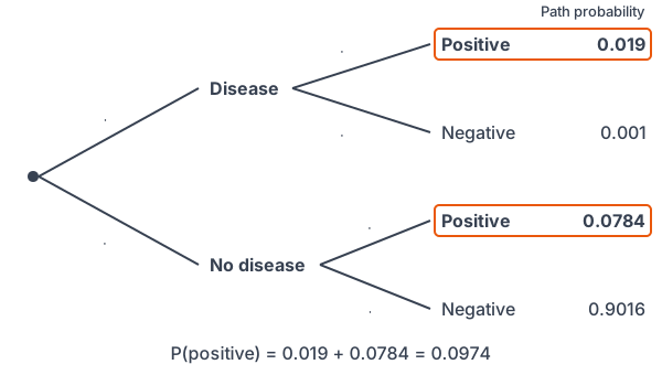
A tree diagram starts with the first event (disease or not) and then the second (test result). Bayes’ theorem works backward from the second event to the first.
Bayes’ theorem formula
P(A \mid B) = \dfrac{P(A) \cdot P(B \mid A)}{P(B)}The bottom, P(B), adds every path in the tree that ends in B. With two branches, A and not A:
P(B) = P(A) \cdot P(B \mid A) + P(A^C) \cdot P(B \mid A^C)
So the steps are: multiply along each branch, add the paths that end in B, then divide the path through A by that total. The first probability, P(A), is sometimes called the prior, and the answer, P(A | B), the posterior.
Bayes’ theorem examples
Example 1: Reverse a tree diagram
In the bus example from the conditional probability lesson, P(bus and late) = 0.09 and P(late) = 0.11. A student is late. Find the probability that the student rode the bus.
P(\text{bus} \mid \text{late}) = \dfrac{P(\text{bus and late})}{P(\text{late})}Write Bayes’ theorem with the path and the total.
P(\text{bus} \mid \text{late}) = \dfrac{0.09}{0.11}Substitute.
\dfrac{0.09}{0.11} \approx 0.818Divide.
Answer: about 0.818. Only 15% of bus riders are late, but about 82% of late students rode the bus, because most students ride the bus and they are late more often.
Example 2: A medical test
A disease affects 2% of people. A test is positive for 95% of people who have the disease and for 8% of people who don’t (false positives). A person tests positive. Find the probability that the person has the disease.
P(\text{D and pos}) = 0.02 \cdot 0.95Multiply along the disease, positive path.
0.02 \cdot 0.95 = 0.019
Multiply (see operations with decimals).
P(\text{no D and pos}) = 0.98 \cdot 0.08Multiply along the no disease, positive path. P(no disease) = 1 − 0.02.
0.98 \cdot 0.08 = 0.0784
Multiply.
P(\text{pos}) = 0.019 + 0.0784Add the paths that end in a positive test.
0.019 + 0.0784 = 0.0974
Add.
P(\text{D} \mid \text{pos}) = \dfrac{0.019}{0.0974}Divide the disease path by the total.
\dfrac{0.019}{0.0974} \approx 0.195Divide.
Answer: about 0.195, or about 20%. Most positive results are false positives, because so many more people don’t have the disease.
Example 3: Check with counts
Redo Example 2 with a group of 10,000 people.
10000 \cdot 0.02 = 200
People with the disease.
200 \cdot 0.95 = 190
Of them, the number who test positive.
10000 - 200 = 9800
People without the disease.
9800 \cdot 0.08 = 784
Of them, the number who test positive.
190 + 784 = 974
Total positive tests.
\dfrac{190}{974} \approx 0.195Share of positives who have the disease.
Answer: 190 of the 974 positive tests come from people with the disease, about 0.195 again. Thinking in counts like this is often the easiest way to see why the answer is low.
Example 4: More than two branches
Factory A makes 50% of a company’s parts, Factory B makes 30% and Factory C makes 20%. Their defect rates are 2%, 3% and 5%. A part is defective. Find the probability that it came from Factory C.
0.50 \cdot 0.02 = 0.010
Path for A and defective.
0.30 \cdot 0.03 = 0.009
Path for B and defective.
0.20 \cdot 0.05 = 0.010
Path for C and defective.
0.010 + 0.009 + 0.010 = 0.029
Add all paths that end in defective.
P(\text{C} \mid \text{defective}) = \dfrac{0.010}{0.029}Divide C’s path by the total.
\dfrac{0.010}{0.029} \approx 0.345Divide.
Answer: about 0.345. Factory C makes only 20% of the parts but about 34% of the defective ones.
Example 5: A spam filter (word problem)
Of the emails a person gets, 40% are spam. The word “prize” appears in 25% of spam emails and in 2% of other emails. An email contains “prize.” Find the probability that it is spam.
0.40 \cdot 0.25 = 0.10
Path for spam and “prize.”
1 - 0.40 = 0.60
Probability an email is not spam (see complement rule).
0.60 \cdot 0.02 = 0.012
Path for not spam and “prize.”
0.10 + 0.012 = 0.112
Total probability of “prize.”
P(\text{spam} \mid \text{prize}) = \dfrac{0.10}{0.112}Divide the spam path by the total.
\dfrac{0.10}{0.112} \approx 0.893Divide.
Answer: about 0.893. Seeing “prize” raises the chance of spam from 40% to about 89%. Real spam filters combine many words this way.
Common mistakes
| Mistake | Example of the error | Fix |
|---|---|---|
| Confusing P(A | B) with P(B | A) | Saying a 95% accurate test means a positive person has a 95% chance of disease | Use Bayes’ theorem: here the answer is about 0.195. |
| Ignoring the base rate | Forgetting that only 2% of people have the disease | Start the tree with P(disease); it changes the answer a lot. |
| Leaving out a path in the total | P(pos) = 0.019 only | Add every path that ends in a positive test: 0.019 + 0.0784. |
| Using the wrong branch for false positives | Using 0.05 (negative, given disease) as the false positive rate | False positives are positive results among people without the disease: 0.08. |
| Dividing by the wrong total | Dividing 0.019 by 1 | Divide by P(B), the total for the event you know happened. |
| Branches that don’t add to 1 | Writing 0.95 and 0.08 as the two branches after disease | Branches from one point add to 1: 0.95 and 0.05. |
Related methods
Two-way tables instead of trees
You can put the counts from Example 3 in a two-way table with rows for disease and columns for test result. Then P(disease | positive) is just the cell divided by the column total, as in conditional probability.
Updating with more evidence
The posterior from one step can be the prior for the next. Practice problem 10 shows how a second positive test raises the probability. If two tests are independent given disease status, you multiply their branch probabilities.
Practice problems
- P(A) = 0.3, P(B | A) = 0.6 and P(B) = 0.4. Find P(A | B).
- Use the bus example (P(no bus and late) = 0.02, P(late) = 0.11). Find P(no bus | late).
- In the bus example, P(bus and on time) = 0.51 and P(on time) = 0.89. Find P(bus | on time).
- A disease affects 1% of people. A test is positive for 90% of people with it and 5% of people without it. Find P(disease | positive).
- Check problem 4 with a group of 10,000 people.
- Use Example 4. Find the probability that a defective part came from Factory B.
- Bag 1 has 3 red and 2 blue marbles. Bag 2 has 1 red and 4 blue. A fair coin picks the bag, and one marble is drawn. It is red. Find P(Bag 1 | red).
- Why can P(disease | positive) be low even when a test is accurate?
- P(A) = 0.5, P(B | A) = 0.2 and P(B | Aᶜ) = 0.6. Find P(B) and P(A | B).
- In Example 2, the person takes the test again and is positive again. Use 0.195 as the new P(disease), and assume the second result is independent of the first given disease status. Find the new P(disease | positive).
Show answers
1.
0.3 \cdot 0.6 = 0.18
Find P(A) · P(B | A).
\dfrac{0.18}{0.4} = 0.45Divide by P(B).
Answer: 0.45
2.
\dfrac{0.02}{0.11} \approx 0.182Divide the path by the total.
Answer: about 0.182
3.
\dfrac{0.51}{0.89} \approx 0.573Divide the path by the total.
Answer: about 0.573
4.
0.01 \cdot 0.90 = 0.009
Disease and positive.
0.99 \cdot 0.05 = 0.0495
No disease and positive.
0.009 + 0.0495 = 0.0585
Total positive.
\dfrac{0.009}{0.0585} \approx 0.154Divide.
Answer: about 0.154
5.
10000 \cdot 0.01 = 100
People with the disease.
100 \cdot 0.90 = 90
Of them, positive.
9900 \cdot 0.05 = 495
People without it who test positive.
90 + 495 = 585
Total positive.
\dfrac{90}{585} \approx 0.154Divide.
Answer: 90 of 585 positives, about 0.154
6.
\dfrac{0.009}{0.029} \approx 0.310Divide B’s path by the total.
Answer: about 0.310
7.
0.5 \cdot \dfrac{3}{5} = 0.3Path for Bag 1 and red.
0.5 \cdot \dfrac{1}{5} = 0.1Path for Bag 2 and red.
0.3 + 0.1 = 0.4
Total for red.
\dfrac{0.3}{0.4} = 0.75Divide.
Answer: 0.75
8.
\text{rare disease}Many more healthy people can test positive by mistake.
Answer: when a disease is rare, false positives from the large healthy group can outnumber true positives
9.
0.5 \cdot 0.2 = 0.1
Path for A and B.
0.5 \cdot 0.6 = 0.3
Path for not A and B.
0.1 + 0.3 = 0.4
P(B).
\dfrac{0.1}{0.4} = 0.25P(A | B).
Answer: P(B) = 0.4 and P(A | B) = 0.25
10.
0.195 \cdot 0.95 = 0.18525
Disease and positive again.
1 - 0.195 = 0.805
New P(no disease).
0.805 \cdot 0.08 = 0.0644
No disease and positive again.
0.18525 + 0.0644 = 0.24965
Total positive.
\dfrac{0.18525}{0.24965} \approx 0.742Divide.
Answer: about 0.742
Bayes’ theorem FAQ
What is Bayes’ theorem in simple terms?
It is a way to update a probability when you get new information. It turns P(B | A), which is often known, into P(A | B), which is often what you want.
What is the formula for Bayes’ theorem?
P(A \mid B) = \dfrac{P(A) \cdot P(B \mid A)}{P(B)}, where P(B) adds every path in the tree that ends in B.
Why do positive tests for rare diseases often turn out false?
When few people have a disease, even a small false positive rate among the many healthy people creates more positives than the sick group does. In Example 2, 784 of 974 positives per 10,000 people are false.
Do I need the formula, or can I use a tree diagram?
A tree diagram gives the same answer. Multiply along each branch, add the paths that end in the known event, and divide the path you want by that total.
Summary
- Bayes’ theorem reverses a conditional probability: it finds P(A | B) from P(B | A).
- Formula: P(A \mid B) = \dfrac{P(A) \cdot P(B \mid A)}{P(B)}.
- Find P(B) by adding every path in the tree that ends in B.
- Counts, like 10,000 people, make the answer easy to check.
- The starting probability, the base rate, matters a lot when an event is rare.
Previous lesson: Independent Events
Next lesson: Discrete Random Variables
Back to the Statistics Index