Discrete Random Variables: Distributions

A discrete random variable is a variable whose value is a number set by chance, with values you can count, like 0, 1, 2 and so on. Its probability distribution lists every possible value with its probability. Each probability is between 0 and 1, and all of them add to 1.

Before this lesson: Probability Rules, Categorical and Quantitative Variables and Dot Plots and Histograms

What is a random variable?

A random variable gives a number to each outcome of a random process. It is usually named with a capital letter like X. For example, flip a coin 3 times and let X be the number of heads. The outcome HTH gives $X = 2$ .

A random variable is discrete if you can list its possible values, such as the number of heads or the number of phones sold. It is continuous if it can take any value in an interval, such as a time or a weight. This lesson covers discrete random variables; continuous ones come with density curves later.

Probability distribution of a discrete random variable

A probability distribution is a table, list or graph of each value $x$ and its probability $P(X = x)$ . It is valid only if both rules hold:

0 \le P(X = x) \le 1

\sum P(X = x) = 1

These are the probability rules again: every probability is between 0 and 1, and they add to 1. The values of X don’t overlap, so to find the chance of a range of values, add their probabilities.

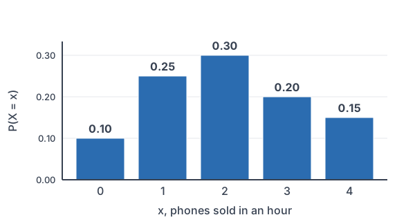
A probability histogram shows the distribution with a bar for each value. The bar heights are the probabilities.

Probability histogram of X, the number of phones a store sells in an hour. Bar heights: 0 phones, 0.10; 1 phone, 0.25; 2 phones, 0.30; 3 phones, 0.20; 4 phones, 0.15. The tallest bar is at 2 phones. — Each bar’s height is a probability, and the five heights add to 1.

Discrete random variable examples

Example 1: Build a distribution

A coin is flipped 3 times. Let X be the number of heads. Find the probability distribution of X.

2^3 = 8

Count the equally likely outcomes (see exponents).

X = 0: \text{TTT}

One outcome has no heads.

X = 1: \text{HTT, THT, TTH}

Three outcomes have 1 head.

X = 2: \text{HHT, HTH, THH}

Three outcomes have 2 heads.

X = 3: \text{HHH}

One outcome has 3 heads.

\dfrac{1}{8} + \dfrac{3}{8} + \dfrac{3}{8} + \dfrac{1}{8} = \dfrac{8}{8}

Check that the probabilities add to 1 (see adding fractions).

x	0	1	2	3
P(X = x)	1/8	3/8	3/8	1/8

Answer: the table above. It is valid, because each probability is between 0 and 1 and they add to 1.

Example 2: Find a missing probability

Let X be the number of pets in a randomly chosen household in a town (example data). Find the missing probability.

x	0	1	2	3	4
P(X = x)	0.32	0.38	0.18	?	0.04

0.32 + 0.38 + 0.18 + 0.04 = 0.92

Add the known probabilities.

1 - 0.92 = 0.08

The probabilities must add to 1.

0 \le 0.08 \le 1

Check that it is a valid probability.

Answer: $P(X = 3) = 0.08$ .

Example 3: Probabilities of ranges

Use the pets distribution from Example 2 (with $P(X = 3) = 0.08$ ). Find the probability that a household has at least 2 pets and the probability that it has fewer than 2.

P(X \ge 2) = 0.18 + 0.08 + 0.04

“At least 2” means 2, 3 or 4.

0.18 + 0.08 + 0.04 = 0.30

Add.

P(X \lt 2) = 0.32 + 0.38

“Fewer than 2” means 0 or 1.

0.32 + 0.38 = 0.70

Add.

0.30 + 0.70 = 1

Check: the two events are complements.

Answer: $P(X \ge 2) = 0.30$ and $P(X \lt 2) = 0.70$ . Watch the words: “at least” includes 2, and “fewer than” does not.

Example 4: Discrete or continuous?

Decide whether each random variable is discrete or continuous: (a) the number of texts a student sends in a day, (b) the time it takes to run a mile, (c) the number of cars in a parking lot at noon.

\text{(a) texts: } 0, 1, 2, \dots

You can list the values, so it is discrete.

\text{(b) time: any value, like } 7.38 \text{ min}

It can be any value in an interval, so it is continuous.

\text{(c) cars: } 0, 1, 2, \dots

Counts are discrete.

Answer: (a) discrete, (b) continuous, (c) discrete. A quick test: counts are discrete, and measurements are continuous.

Example 5: Phones sold per hour (word problem)

A phone store tracks X, the number of phones it sells in an hour (example data):

x	0	1	2	3	4
P(X = x)	0.10	0.25	0.30	0.20	0.15

Find the probability that the store sells at least one phone, between 2 and 3 phones (inclusive), and more than 2 phones.

P(X \ge 1) = 1 - P(X = 0)

Use the complement of selling none.

1 - 0.10 = 0.90

Subtract.

P(2 \le X \le 3) = 0.30 + 0.20

Add the values 2 and 3.

0.30 + 0.20 = 0.50

Add.

P(X \gt 2) = 0.20 + 0.15

“More than 2” means 3 or 4.

0.20 + 0.15 = 0.35

Add.

Answer: 0.90, 0.50 and 0.35. The histogram above shows this distribution. The next lesson, Expected Value, finds the average number of phones sold per hour.

Common mistakes

Mistake	Example of the error	Fix
Probabilities that don’t add to 1	A table with 0.2, 0.3, 0.4 and 0.2	Add them: they total 1.1, so the table is not valid.
Mixing up “at least” and “more than”	Using 3 and 4 for P(X ≥ 2)	“At least 2” includes 2; “more than 2” doesn’t.
Adding the values instead of the probabilities	P(X ≥ 2) = 2 + 3 + 4	Add the probabilities of those values: 0.18 + 0.08 + 0.04.
Calling a measurement discrete	Saying running time is discrete because the watch shows whole seconds	Time can take any value in an interval, so it is continuous.
Skipping outcomes when building a distribution	Listing only HHT for X = 2	List every outcome: HHT, HTH and THH.
Confusing X with x	Writing P(x) for the random variable itself	X is the random variable; x is one of its values.

Related methods

Probability histograms and data histograms

A probability histogram looks like the data histograms in dot plots and histograms, but its heights are probabilities instead of counts. You can describe its shape, center and spread the same way as in describing a distribution.

Adding probabilities of values

Different values of X can’t happen at once, so they are mutually exclusive. That is why you add their probabilities, as in the addition rule. For “at least one,” the complement is often faster.

Practice problems

Is this a valid probability distribution: P(X = 1) = 0.2, P(X = 2) = 0.3, P(X = 3) = 0.4, P(X = 4) = 0.2? Explain.
A distribution has P(X = 0) = 0.15, P(X = 1) = 0.4, P(X = 3) = 0.1, and X can also be 2. Find P(X = 2).
A coin is flipped 2 times. Let X be the number of heads. Find the distribution of X.
Use the pets distribution from Example 3. Find P(X ≤ 1).
Use the pets distribution. Find P(1 ≤ X ≤ 3).
Is the weight of a backpack discrete or continuous?
Is the number of siblings a student has discrete or continuous?
A die is rolled. Let X be the number rolled. Find P(X > 4).
Use the phone store distribution in Example 5. Find P(X < 3).
Two dice are rolled. Let X be the sum. Find P(X = 7) and P(X ≥ 11).

Show answers

0.2 + 0.3 + 0.4 + 0.2 = 1.1

Add the probabilities.

Answer: no, because the probabilities add to 1.1, not 1

0.15 + 0.4 + 0.1 = 0.65

Add the known probabilities.

1 - 0.65 = 0.35

Subtract from 1.

Answer: 0.35

2^2 = 4

Count the outcomes: HH, HT, TH, TT.

P(X = 0) = \dfrac{1}{4}

Only TT.

P(X = 1) = \dfrac{2}{4} = \dfrac{1}{2}

HT and TH.

P(X = 2) = \dfrac{1}{4}

Only HH.

Answer: X = 0, 1, 2 with probabilities 1/4, 1/2, 1/4

0.32 + 0.38 = 0.70

Add the values 0 and 1.

Answer: 0.70

0.38 + 0.18 + 0.08 = 0.64

Add the values 1, 2 and 3.

Answer: 0.64

\text{weight is measured}

It can be any value in an interval.

Answer: continuous

\text{siblings are counted}

The values are 0, 1, 2 and so on.

Answer: discrete

\text{values 5 and 6}

“Greater than 4” means 5 or 6.

\dfrac{1}{6} + \dfrac{1}{6} = \dfrac{2}{6}

Add.

\dfrac{2}{6} = \dfrac{1}{3}

Simplify.

Answer: 1/3

0.10 + 0.25 + 0.30 = 0.65

Add the values 0, 1 and 2.

Answer: 0.65

10.

\dfrac{6}{36} = \dfrac{1}{6}

Six of the 36 outcomes have a sum of 7.

\text{11: (5,6), (6,5); 12: (6,6)}

List the outcomes with a sum of 11 or 12.

\dfrac{3}{36} = \dfrac{1}{12}

Divide and simplify.

Answer: P(X = 7) = 1/6 and P(X ≥ 11) = 1/12

Discrete random variable FAQ

What is a discrete random variable?

It is a random variable with values you can list or count, like the number of heads in 3 flips. Each value has a probability.

What makes a probability distribution valid?

Every probability must be between 0 and 1, and all the probabilities must add to exactly 1.

What is the difference between discrete and continuous random variables?

Discrete random variables take countable values, usually counts. Continuous random variables can take any value in an interval, usually measurements like time, height or weight.

How do you find P(X ≥ a) from a table?

Add the probabilities of every value that is a or larger. If that list is long, subtract the probabilities of the smaller values from 1 instead.

Summary

A random variable X assigns a number to each outcome of a random process.
Discrete random variables have countable values; continuous ones take any value in an interval.
A probability distribution lists each value with its probability.
Valid distributions: each probability is between 0 and 1, and they add to 1.
For a range of values, add their probabilities, or use the complement.

Previous lesson: Bayes’ Theorem

Next lesson: Expected Value

Back to the Statistics Index