
Categorical and Quantitative Variables
A categorical variable places each individual into a group, such as eye color or favorite sport. A quantitative variable is a number you measure or count, such as height or number of siblings, where an average makes sense. The type decides the graph: bar or pie charts for categorical data; dot plots, histograms or box plots for quantitative data.
Before this lesson: Mean, Median, Mode and Range, Dot Plots and Histograms and Two-Way Tables
Individuals and variables
Data describe individuals: the people, animals or things you collect information about. A variable is one characteristic you record for each individual, and it can take different values. In a data table, each row is usually an individual and each column is a variable.
The first question about any variable is what kind it is. A quick test: would it make sense to average the values? If yes, the variable is quantitative. If the values are labels or groups, it is categorical, even when the labels are numbers, like zip codes.
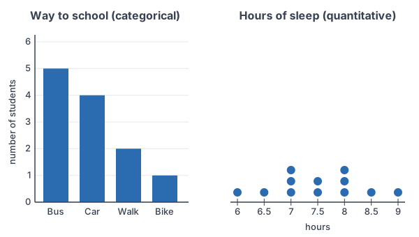
Categorical vs. quantitative variables
| Categorical variable | Quantitative variable | |
|---|---|---|
| Values | Groups or labels | Numbers from measuring or counting |
| Examples | Eye color, blood type, zip code, yes/no answer | Height, age, test score, number of texts |
| Does an average make sense? | No | Yes |
| How to summarize | Counts and percents in each group | Center (mean, median) and spread (range, IQR, standard deviation) |
| Graphs | Bar chart, pie chart | Dot plot, histogram, stem-and-leaf plot, box plot |
Two kinds of quantitative variables
- A discrete quantitative variable comes from counting, so it has gaps between possible values: number of siblings, goals scored.
- A continuous quantitative variable comes from measuring, so any value in a range is possible: time, weight, temperature.
- Some categorical variables have a natural order, like letter grades or survey answers from “strongly disagree” to “strongly agree.” They are still categorical.
How to classify a variable
- Name the individuals and the variable.
- Look at the values. Are they groups or labels, or are they amounts?
- Ask whether an average would mean something.
- If it is quantitative, decide whether it is counted (discrete) or measured (continuous).
Categorical and quantitative variable examples
Example 1: Classify every variable in a table
A class survey records these values (example data). Name the individuals, and classify each variable.
| Student | Way to school | Hours of sleep | Apps on phone | Favorite subject |
|---|---|---|---|---|
| Ana | Bus | 7.5 | 42 | Biology |
| Ben | Car | 6 | 65 | History |
| Cara | Walk | 8 | 38 | Algebra |
| Dev | Bus | 7 | 51 | Art |
\text{Individuals: the 4 students}Each row describes one student.
\text{Way to school: categorical}Its values (bus, car, walk) are groups.
\text{Hours of sleep: quantitative}Its values are measured amounts, and an average like 7.1 hours makes sense.
\text{Apps on phone: quantitative}Its values are counts, and an average number of apps makes sense.
\text{Favorite subject: categorical}Its values are names of subjects.
Answer: the individuals are the students. Way to school and favorite subject are categorical; hours of sleep and apps on phone are quantitative. The name column only identifies each student.
Example 2: Numbers that are really labels
Classify each variable: a person’s zip code, a player’s jersey number, a runner’s age in years, and a survey answer coded 1 = yes, 2 = no.
\text{Zip code: categorical}It names a place. An “average zip code” means nothing.
\text{Jersey number: categorical}It is a label; player 24 is not “twice” player 12.
\text{Age in years: quantitative}It is an amount of time, and an average age makes sense.
\text{Yes/no answer coded 1 or 2: categorical}The codes stand for groups. Averaging them to 1.4 means nothing.
Answer: only age is quantitative. Being written as a number is not enough; ask whether arithmetic on the values means something.
Example 3: Discrete or continuous?
Classify each quantitative variable as discrete or continuous: number of texts sent today, time spent on a phone today, weight of a backpack, number of siblings.
\text{Texts sent: discrete}You count texts: 0, 1, 2, … with nothing between.
\text{Time on phone: continuous}You measure time; 2.37 hours is possible.
\text{Backpack weight: continuous}You measure weight, so any value in a range is possible.
\text{Number of siblings: discrete}You count siblings.
Answer: counts (texts, siblings) are discrete; measurements (time, weight) are continuous.
Example 4: Summarize each type
For the 12 students in the graph above (example data), 5 ride the bus, 4 come by car, 2 walk and 1 bikes. Their hours of sleep are 6, 6.5, 7, 7, 7, 7.5, 7.5, 8, 8, 8, 8.5 and 9. Summarize each variable in a way that fits its type.
\dfrac{5}{12} \approx 0.417 = 41.7\%Way to school is categorical, so find the percent in each group. Divide the count by the total (see percentages).
\dfrac{4}{12} \approx 33.3\%, \; \dfrac{2}{12} \approx 16.7\%, \; \dfrac{1}{12} \approx 8.3\%Repeat for car, walk and bike.
\bar{x} = \dfrac{\sum x}{n}Sleep is quantitative, so find its mean: add the values and divide by how many there are.
\sum x = 6 + 6.5 + 7 + 7 + 7 + 7.5 + 7.5 + 8 + 8 + 8 + 8.5 + 9 = 90
Add the 12 values.
\bar{x} = \dfrac{90}{12} = 7.5Divide by n = 12.
On a TI-84: press STAT, choose 1:Edit and type the 12 sleep values into L1. Then press STAT, arrow right to CALC, choose 1:1-Var Stats and press ENTER. The screen shows x̄ = 7.5 and n = 12.
In Desmos: type s = [6, 6.5, 7, 7, 7, 7.5, 7.5, 8, 8, 8, 8.5, 9] on one line and mean(s) on the next. Desmos shows 7.5.
Answer: 41.7% ride the bus, 33.3% come by car, 16.7% walk and 8.3% bike. The mean sleep time is 7.5 hours. A mean of the way-to-school values would make no sense.
Example 5: One question, two variables (word problem)
A health survey asks 300 adults how many hours they exercise each week. The researchers record the exact hours, then also sort each person into “less than 2 hours,” “2 to 5 hours” or “more than 5 hours.” Classify both variables, and choose a graph for each.
\text{Exact hours per week: quantitative (continuous)}It is a measured amount of time, so an average makes sense.
\text{Exercise group: categorical}Each person is placed in one of three groups.
\text{Hours: histogram or box plot}Quantitative data go on a number line.
\text{Groups: bar chart or pie chart}Categorical data are shown as counts or percents.
Answer: the same question can produce a quantitative variable (the hours) and a categorical variable (the group). Grouping loses detail, since 2.1 and 4.9 hours land in the same group.
Common mistakes
| Mistake | Example of the error | Fix |
|---|---|---|
| Calling every number quantitative | “Zip code is quantitative because it is a number” | Ask whether an average makes sense. For zip codes it doesn’t, so they are categorical. |
| Averaging category codes | Coding bus = 1, car = 2, walk = 3 and finding a mean of 1.75 | Codes are labels. Summarize with counts and percents. |
| Using a histogram for categorical data | Drawing touching bars for way to school | Use a bar chart with gaps, or a pie chart. Histograms are for quantitative data. |
| Mixing up the variable and its values | Calling “bus” a variable | The variable is way to school; bus is one of its values. |
| Thinking counts of a group make the variable quantitative | “5 students ride the bus, so way to school is quantitative” | The count summarizes a categorical variable. The variable itself is still categorical. |
| Thinking quantitative values must be decimals | “Number of siblings is categorical because it is a whole number” | Counts are quantitative (discrete). An average of 1.8 siblings makes sense. |
Related methods
Two variables at once
When you study two categorical variables together, such as grade level and favorite sport, organize them in a two-way table. When both variables are quantitative, such as hours studied and test score, plot them in a scatter plot.
Graphing each type
Quantitative data use number-line graphs, such as dot plots and histograms and box plots. Categorical data use bar graphs and pie charts, the topic of the next lesson.
Practice problems
- Classify the variable: a student’s favorite music genre.
- Classify the variable: a person’s height in centimeters. If it is quantitative, is it discrete or continuous?
- Classify the variable: a phone number’s area code.
- Classify the variable: the number of pets in a household. Discrete or continuous?
- Classify the variable: a student’s letter grade (A, B, C, D or F).
- A table lists all 50 U.S. states with each state’s region, population and number of national parks. Name the individuals and classify each variable.
- A survey asks 80 students for their favorite school lunch. Which graphs would work for the results?
- In a survey of 60 students, 18 walk to school. What percent walk?
- Five commute times, in minutes, are 12, 18, 25, 9 and 16. Find the mean by hand, and give the TI-84 or Desmos steps.
- A basketball coach records each player’s position (guard, forward, center) and vertical jump in inches. Classify each variable and choose a graph and a summary for each.
Show answers
1.
\text{Favorite genre: categorical}The values (pop, rock, country, …) are groups.
Answer: categorical
2.
\text{Height: quantitative}Height is a measured amount, and an average makes sense.
\text{Height: continuous}It is measured, so values like 171.4 cm are possible.
Answer: quantitative, continuous
3.
\text{Area code: categorical}It labels a region; an average area code means nothing.
Answer: categorical
4.
\text{Number of pets: quantitative}It is a count, and an average like 1.6 pets makes sense.
\text{Number of pets: discrete}You count pets: 0, 1, 2, …
Answer: quantitative, discrete
5.
\text{Letter grade: categorical}The grades are ordered groups, not amounts.
Answer: categorical (with a natural order)
6.
\text{Individuals: the 50 states}Each row describes one state.
\text{Region: categorical; population, national parks: quantitative}Region names a group; population and park counts are amounts.
Answer: individuals are the states; region is categorical; population and number of national parks are quantitative (discrete)
7.
\text{Favorite lunch: categorical}The answers are groups.
Answer: a bar chart or a pie chart of the counts or percents
8.
\dfrac{18}{60} = 0.30Divide the count by the total.
0.30 = 30\%
Change the decimal to a percent.
Answer: 30%
9.
\sum x = 12 + 18 + 25 + 9 + 16 = 80
Add the five times.
\bar{x} = \dfrac{80}{5} = 16Divide by n = 5.
\text{TI-84: STAT, 1:Edit, enter in L1; STAT, CALC, 1:1-Var Stats}The screen shows x̄ = 16. In Desmos, type t = [12, 18, 25, 9, 16] and then mean(t).
Answer: the mean commute is 16 minutes
10.
\text{Position: categorical; vertical jump: quantitative}Position is a group; jump height is a measured amount.
\text{Position: counts and a bar chart}Count the players at each position.
\text{Jump: mean or median and a dot plot or histogram}Summarize center and spread on a number line.
Answer: position is categorical (bar chart, counts); vertical jump is quantitative and continuous (dot plot or histogram, mean or median)
Categorical and quantitative variables FAQ
What is the difference between categorical and quantitative variables?
A categorical variable puts individuals into groups, such as blood type. A quantitative variable records a number from measuring or counting, such as weight, where an average makes sense.
Is age a categorical or quantitative variable?
Age in years is quantitative, because an average age makes sense. If ages are grouped into ranges like 18–24 and 25–34, the age group is categorical.
Is a zip code categorical or quantitative?
Categorical. A zip code is a label for a place, and adding or averaging zip codes means nothing.
What graphs go with each type of variable?
Use bar charts or pie charts for categorical variables. Use dot plots, histograms, stem-and-leaf plots or box plots for quantitative variables.
Summary
- Individuals are what the data describe; variables are what you record about each one.
- Categorical variables place individuals in groups; quantitative variables are measured or counted amounts.
- Test: if an average makes sense, the variable is quantitative.
- Quantitative variables are discrete (counted) or continuous (measured).
- Summarize categorical data with counts and percents; summarize quantitative data with center and spread.
Previous course: Calculus 2 Index
Next lesson: Bar Graphs and Pie Charts
Back to the Statistics Index