Describing a Distribution: SOCS Examples

Describing a distribution means telling what the graph of a quantitative variable shows: its shape, any outliers, its center and its spread, written in the context of the data. A short way to remember this is SOCS. For example: “Commute times are skewed right, with a median of 27.5 minutes and a range of 21 minutes.”

Before this lesson: Dot Plots and Histograms, Stem-and-Leaf Plots, Box Plots and Mean, Median, Mode and Range

What it means to describe a distribution

The distribution of a variable tells what values it takes and how often it takes them. A dot plot, histogram or stem-and-leaf plot is a picture of a distribution.

To describe one, answer four questions, always using the variable’s name and units. What is the overall shape? Are there outliers? Where is the middle? How spread out are the values? A good description reads like a sentence about the real situation, not a list of numbers.

Four small example histograms showing common shapes. Symmetric: bars rise to a single peak in the middle and fall evenly on both sides. Skewed right: the peak is on the left and a long tail stretches to the right. Skewed left: the peak is on the right and a long tail stretches to the left. Bimodal: two separate peaks with a dip between them. — Common shapes. A skewed distribution is named for the side its long tail points to, not for its peak.

SOCS: shape, outliers, center and spread

Feature	What to look for	Words to use
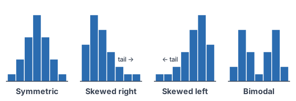
Shape	Peaks, symmetry and tails	Symmetric, skewed right, skewed left, uniform, unimodal (one peak), bimodal (two peaks)
Outliers	Values far from the rest, often after a gap	“A possible outlier at 85 bpm”; also mention gaps and clusters
Center	The typical value	Median, or mean if the shape is roughly symmetric with no outliers
Spread	How far the values reach and how tightly they bunch	Range, IQR, or standard deviation

How the shape decides the summary

In a skewed right distribution, the long tail is toward larger values, and the mean is usually greater than the median.
In a skewed left distribution, the long tail is toward smaller values, and the mean is usually less than the median.
In a symmetric distribution, the mean and median are close.
For skewed data or data with outliers, report the median and the interquartile range (IQR), because they are resistant: extreme values barely change them. For roughly symmetric data, the mean and standard deviation work well.

Describing a distribution examples

Example 1: Use the mean and median to see skew

Twenty-five students report their number of siblings (example data): 0 siblings 4 students, 1 sibling 9, 2 siblings 6, 3 siblings 3, 4 siblings 2 and 6 siblings 1. Find the mean and median, and describe the shape.

n = 4 + 9 + 6 + 3 + 2 + 1 = 25

Add the counts to check the total.

\dfrac{25 + 1}{2} = 13

The median is the 13th value (see mean, median, mode and range).

4 + 9 = 13

The 0s fill positions 1 to 4, and the 1s fill positions 5 to 13.

\text{Median} = 1

So the 13th value is 1.

\textstyle\sum x = 0(4) + 1(9) + 2(6) + 3(3) + 4(2) + 6(1)

Multiply each value by its count to add all 25 values.

\textstyle\sum x = 0 + 9 + 12 + 9 + 8 + 6 = 44

Simplify.

\bar{x} = \dfrac{44}{25} = 1.76

Divide by n.

1.76 \gt 1

The mean is greater than the median.

Answer: the median is 1 sibling and the mean is 1.76 siblings. The peak is at 1 and the values trail off toward 6, so the distribution is skewed right. The long right tail pulls the mean above the median.

Example 2: Write a full SOCS description (word problem)

The resting heart rates, in beats per minute (bpm), of 15 athletes are (example data): 48, 52, 55, 56, 58, 59, 60, 61, 61, 62, 63, 64, 66, 68, 85. Describe the distribution.

4 \mid 8, \; 5 \mid 2 \; 5 \; 6 \; 8 \; 9, \; 6 \mid 0 \; 1 \; 1 \; 2 \; 3 \; 4 \; 6 \; 8, \; 7 \mid \;, \; 8 \mid 5

Make a quick stemplot to see the shape. Row 7 is empty.

\text{Median} = 8\text{th value} = 61

With 15 values, the median is the 8th.

\text{Lower half: } 48, 52, 55, 56, 58, 59, 60 \Rightarrow Q_1 = 56

Q1 is the median of the 7 values below the median.

\text{Upper half: } 61, 62, 63, 64, 66, 68, 85 \Rightarrow Q_3 = 64

Q3 is the median of the 7 values above the median.

\text{IQR} = Q_3 - Q_1 = 64 - 56 = 8

Subtract to find the IQR (see box plots).

\text{Range} = 85 - 48 = 37

Largest minus smallest.

\bar{x} = \dfrac{918}{15} = 61.2

The mean, for comparison; the 15 values add to 918.

On a TI-84: enter the values in L1, then STAT, CALC, 1:1-Var Stats. Scroll to see x̄ = 61.2, Q1 = 56, Med = 61 and Q3 = 64. In Desmos: $h = [48, 52, 55, 56, 58, 59, 60, 61, 61, 62, 63, 64, 66, 68, 85]$ , then median(h) and mean(h).

Answer: Shape: roughly symmetric with one peak in the low 60s, apart from one high value. Outliers: 85 bpm sits far above the rest, after a gap of 17 bpm, so it is a possible outlier. Center: the median resting heart rate is 61 bpm. Spread: the middle half of the athletes are within an IQR of 8 bpm; the full range is 37 bpm.

Example 3: Choose the best measure of center

Five homes on a street sold for (example data) $210,000, $225,000, $240,000, $260,000 and $900,000. Which better describes a typical price, the mean or the median?

210 + 225 + 240 + 260 + 900 = 1835

Work in thousands of dollars. Add the prices.

\bar{x} = \dfrac{1835}{5} = 367

Divide by 5.

\text{Median} = 240

The middle (3rd) of the 5 ordered prices.

367 \gt 260

The mean is larger than four of the five prices.

Answer: the median, $240,000. The one $900,000 home skews the data right and pulls the mean up to $367,000, which is not typical of this street.

Example 4: Predict the shape from the context

Predict the shape of each distribution: (a) scores on a very easy quiz, (b) the number of pets in each household in a town, (c) the heights of a large group of adult women, (d) the heights of a group of 1st graders and their parents.

\text{(a) Skewed left}

Most scores are high, near the top of the scale; a few low scores make a tail to the left.

\text{(b) Skewed right}

Most households have 0, 1 or 2 pets; a few have many, making a tail to the right.

\text{(c) Symmetric}

Most heights are near the middle, with fewer very short or very tall women.

\text{(d) Bimodal}

Children and adults form two separate groups, so the graph has two peaks.

Answer: skewed left, skewed right, symmetric and bimodal. A bimodal shape is often a sign that two different groups are mixed together.

Example 5: A uniform distribution

A die is rolled 60 times (example data). The counts for faces 1 to 6 are 9, 11, 10, 10, 8 and 12. Describe the distribution.

9 + 11 + 10 + 10 + 8 + 12 = 60

Check the total.

\textstyle\sum x = 1(9) + 2(11) + 3(10) + 4(10) + 5(8) + 6(12)

Multiply each face by its count.

\textstyle\sum x = 9 + 22 + 30 + 40 + 40 + 72 = 213

Simplify.

\bar{x} = \dfrac{213}{60} = 3.55

Divide by n = 60.

9 + 11 + 10 = 30

Faces 1 to 3 fill positions 1 to 30, so the 30th roll is a 3 and the 31st is a 4.

\text{Median} = \dfrac{3 + 4}{2} = 3.5

With 60 values, average the 30th and 31st.

\text{Range} = 6 - 1 = 5

Largest minus smallest face.

Answer: the shape is roughly uniform (all bars about the same height, 8 to 12), with no outliers. The center is about 3.5 (median 3.5, mean 3.55), and the rolls spread over the full range of 5, from 1 to 6.

Common mistakes

Mistake	Example of the error	Fix
Naming skew by the peak	Calling a graph with its peak on the right “skewed right”	Skew is named for the tail. A peak on the right with a tail to the left is skewed left.
Leaving out context	“It is skewed right with a median of 61.”	Name the variable and units: “The median resting heart rate is 61 bpm.”
Using the mean and range for skewed data	Reporting a mean home price of $367,000 for Example 3	For skewed data or outliers, report the median and IQR.
Listing numbers without describing	“Median 61, IQR 8, range 37.”	Write sentences that cover shape, outliers, center and spread.
Calling every large value an outlier	Calling 68 bpm an outlier because it is the second highest	Look for a clear gap; the 1.5 × IQR rule gives a formal test.
Saying a variable “is normal” from a small sample	“The 15 heart rates are normally distributed.”	Say “roughly symmetric” unless you have a reason to claim more.

Related methods

Measures of spread

The IQR, the spread of the middle half of the data, comes from the five-number summary used in box plots. The standard deviation, which measures the typical distance from the mean, is the topic of the next lesson.

Outliers and comparing groups

The 1.5 × IQR rule gives an exact cutoff for outliers, and comparing distributions uses SOCS for two or more groups at once. Both come later in this unit. To graph the data first, use a dot plot or histogram or a stem-and-leaf plot.

Practice problems

A histogram has its peak on the right and a long tail stretching to the left. What is its shape?
A data set has a mean of 42 and a median of 35. What shape is it most likely to have?
Find the mean and median of 3, 4, 4, 5, 5, 5, 6, 6, 7, and describe the shape.
Values 1, 2, 3, 4 and 5 occur 2, 5, 8, 5 and 2 times. Find the mean and median.
Find the median, Q1, Q3 and IQR of 10, 12, 15, 18, 20, 22, 25, 30, 41.
Starting salaries at a company are strongly skewed right. Which measures of center and spread should a report use?
A data set lists the heights of a group of jockeys and a group of basketball players. What shape would a histogram most likely have?
Describe the distribution of these 16 commute times, in minutes: 20, 22, 23, 24, 25, 25, 26, 27, 28, 29, 31, 31, 32, 34, 36, 41.
The data 4, 5, 6, 7, 8 have mean 6 and median 6. If 8 is changed to 38, what are the new mean and median?
A four-color spinner is spun 40 times and lands on each color 10, 9, 11 and 10 times. Describe the shape.

Show answers

\text{Tail on the left}

Skew is named for the side of the long tail.

Answer: skewed left

42 \gt 35

The mean is greater than the median.

\text{Mean pulled up by a right tail}

Large values pull the mean up more than the median.

Answer: skewed right

3 + 4 + 4 + 5 + 5 + 5 + 6 + 6 + 7 = 45

Add the 9 values.

\bar{x} = \dfrac{45}{9} = 5

Divide by 9.

\text{Median} = 5

The middle (5th) value is 5.

Answer: mean 5 and median 5; the values are symmetric around 5

n = 2 + 5 + 8 + 5 + 2 = 22

Add the counts.

\textstyle\sum x = 1(2) + 2(5) + 3(8) + 4(5) + 5(2) = 66

Add value × count: 2 + 10 + 24 + 20 + 10.

\bar{x} = \dfrac{66}{22} = 3

Divide by n.

2 + 5 = 7, \; 7 + 8 = 15

The 3s fill positions 8 to 15, which include the 11th and 12th.

\text{Median} = \dfrac{3 + 3}{2} = 3

Average the 11th and 12th values.

Answer: mean 3, median 3 (a symmetric shape)

\text{Median} = 20

The 5th of 9 values.

Q_1 = \dfrac{12 + 15}{2} = 13.5

Median of the lower half 10, 12, 15, 18.

Q_3 = \dfrac{25 + 30}{2} = 27.5

Median of the upper half 22, 25, 30, 41.

\text{IQR} = 27.5 - 13.5 = 14

Subtract Q1 from Q3.

Answer: median 20, Q1 = 13.5, Q3 = 27.5, IQR = 14

\text{Skewed data} \Rightarrow \text{resistant measures}

The median and IQR are not pulled by the long tail of high salaries.

Answer: the median and the IQR

\text{Two groups with different typical heights}

Jockeys are short and basketball players are tall.

Answer: bimodal, with one peak for each group

\text{Median} = \dfrac{27 + 28}{2} = 27.5

With 16 values, average the 8th and 9th.

\text{Range} = 41 - 20 = 21

Largest minus smallest.

\text{Peak at 25 to 29; tail to 41}

Most times are in the 20s, with fewer long commutes.

Answer: commute times are skewed right, with no clear outliers; the median commute is 27.5 minutes, and times range over 21 minutes, from 20 to 41

4 + 5 + 6 + 7 + 38 = 60

Add the new values.

\bar{x} = \dfrac{60}{5} = 12

Divide by 5.

\text{Median} = 6

The middle value is still 6.

Answer: the mean jumps to 12, but the median stays 6; the median is resistant

10.

\text{Counts } 10, 9, 11, 10

All four bars are about the same height.

Answer: roughly uniform; each color comes up about equally often

Describing a distribution FAQ

What does SOCS stand for in statistics?

SOCS stands for shape, outliers, center and spread, the four features to describe for any quantitative distribution. Always describe them in the context of the data.

How do you tell if a distribution is skewed right or left?

Look at the tail. If the long tail stretches toward larger values, it is skewed right; if it stretches toward smaller values, it is skewed left. In right-skewed data the mean is usually greater than the median.

Should you use the mean or the median for skewed data?

Use the median, and the IQR for spread. Extreme values in the tail pull the mean and the standard deviation, but barely change the median and the IQR.

What is a bimodal distribution?

A bimodal distribution has two clear peaks. It often means the data mix two groups, such as children and adults.

Summary

Describe a distribution with SOCS: shape, outliers, center and spread, always in context with units.
Shapes: symmetric, skewed right (tail to larger values), skewed left (tail to smaller values), uniform and bimodal.
Skewed right usually means mean > median; skewed left usually means mean < median.
Use the median and IQR for skewed data or outliers; the mean and standard deviation for roughly symmetric data.
Point out gaps, clusters and possible outliers.

Previous lesson: Stem-and-Leaf Plots

Next lesson: Standard Deviation

Back to the Statistics Index