Comparing Distributions in Statistics

Comparing distributions means describing how two or more groups differ in shape, outliers, center and spread, using comparison words and the context. Graph the groups on the same scale, then write sentences like “Route 1’s median time is 2 minutes longer than Route 2’s, but its IQR is less than half as large.”

Before this lesson: Describing a Distribution, Box Plots, Stem-and-Leaf Plots and Standard Deviation

What it means to compare distributions

Describing one distribution uses SOCS: shape, outliers, center and spread. Comparing two distributions uses the same four features, but every statement must say how the groups differ. Words like “greater than,” “less than,” “about the same as” and “more variable than” do the work.

A fair comparison needs graphs on the same scale: side-by-side box plots, dot plots stacked on one number line, a back-to-back stemplot, or histograms with matching axes. When the groups have different sizes, compare percents or relative frequencies, not counts.

Side-by-side box plots of example travel times in minutes on one scale from 10 to 55. Route 1: minimum 18, Q1 22, median 25, Q3 28, maximum 34. Route 2: minimum 15, Q1 20, median 23, Q3 33, maximum 52, with a long right whisker. — Route 2 has a slightly lower median but a much wider box and a long right tail, so its times are less predictable.

How to compare distributions

Graph the groups on the same scale.
Shape: compare the shapes (for example, “Route 1 is roughly symmetric, while Route 2 is skewed right”).
Outliers: say which group has outliers or gaps, if any.
Center: compare the medians (or means), saying which is greater and by about how much.
Spread: compare the IQRs (or standard deviations, or ranges) and say which group is more variable.
Use the same kind of measure for both groups, and always include the context and units.

Use medians and IQRs when either group is skewed or has outliers. Use means and standard deviations only when both groups are roughly symmetric with no outliers.

Comparing distributions examples

Example 1: Compare two five-number summaries

Quiz scores for two classes (example data) have these five-number summaries. Class A: 52, 68, 76, 82, 95. Class B: 60, 72, 81, 85, 92. Compare the distributions.

81 - 76 = 5

Compare the medians: Class B’s is 5 points higher.

\text{IQR}_A = 82 - 68 = 14, \; \text{IQR}_B = 85 - 72 = 13

Compare the IQRs (see box plots).

\text{Range}_A = 95 - 52 = 43, \; \text{Range}_B = 92 - 60 = 32

Compare the ranges.

68 - 1.5(14) = 47, \; 82 + 1.5(14) = 103

Class A’s fences: 52 and 95 are inside them.

72 - 1.5(13) = 52.5, \; 85 + 1.5(13) = 104.5

Class B’s fences: 60 and 92 are inside them.

Answer: Class B’s median score (81) is 5 points higher than Class A’s (76). The middle halves are about equally spread (IQRs 13 and 14), but Class A’s scores cover a wider range (43 vs. 32 points) because of its low minimum. Neither class has outliers by the 1.5 × IQR rule.

Example 2: Same center, different spread

Two brands of batteries are tested (example data). Brand X lasts 10, 12, 11, 13 and 14 hours. Brand Y lasts 8, 15, 12, 9 and 16 hours. Compare them with the mean and standard deviation.

\bar{x}_X = \dfrac{60}{5} = 12, \; \bar{x}_Y = \dfrac{60}{5} = 12

Both brands’ values add to 60, so both means are 12 hours.

\text{X: } 4 + 0 + 1 + 1 + 4 = 10

Squared deviations from 12 for Brand X.

s_X = \sqrt{\dfrac{10}{4}} \approx 1.58

Divide by n − 1 = 4 and take the root (see standard deviation).

\text{Y: } 16 + 9 + 0 + 9 + 16 = 50

Squared deviations from 12 for Brand Y.

s_Y = \sqrt{\dfrac{50}{4}} \approx 3.54

Divide by 4 and take the root.

Answer: both brands last 12 hours on average, but Brand Y’s battery life is more than twice as variable (standard deviation about 3.54 hours vs. 1.58 hours). Brand X is more consistent.

Example 3: Side-by-side box plots (word problem)

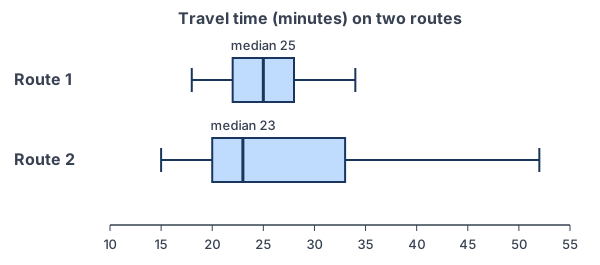
A commuter times two routes to work on many days (example data). The five-number summaries are Route 1: 18, 22, 25, 28, 34 minutes and Route 2: 15, 20, 23, 33, 52 minutes. Which route should she take?

25 - 23 = 2

Center: Route 1’s median is 2 minutes longer.

\text{IQR}_1 = 28 - 22 = 6, \; \text{IQR}_2 = 33 - 20 = 13

Spread: Route 2’s IQR is more than twice as large.

52 - 33 = 19 \gt 23 - 15 = 8

Shape: Route 2’s right whisker is much longer than its left, so it is skewed right.

33 + 1.5(13) = 52.5 \gt 52

Outliers: 52 is just inside Route 2’s upper fence, so no outliers.

Answer: Route 2 is a little faster on a typical day (median 23 vs. 25 minutes), but its times are much more variable (IQR 13 vs. 6 minutes) and skewed right, with some trips near 52 minutes. If she must arrive on time, Route 1 is the safer choice.

Example 4: Choose measures when one group has an outlier

Hours of sleep for two small groups (example data): Group A: 6, 7, 7, 8, 8, 9. Group B: 5, 6, 6, 7, 7, 13. Which measure of center should you compare?

Q_1 = 6, \; Q_3 = 7 \text{ for B}

Group B’s lower half is 5, 6, 6 and its upper half is 7, 7, 13.

\text{IQR}_B = 1, \; 7 + 1.5(1) = 8.5

Find B’s upper fence.

13 \gt 8.5

So 13 hours is an outlier in Group B.

\text{Median}_A = \dfrac{7 + 8}{2} = 7.5, \; \text{Median}_B = \dfrac{6 + 7}{2} = 6.5

Compare medians, which resist the outlier.

\bar{x}_A = \dfrac{45}{6} = 7.5, \; \bar{x}_B = \dfrac{44}{6} \approx 7.33

The means look close only because 13 pulls B’s mean up.

Answer: compare medians. Group A’s median sleep (7.5 hours) is 1 hour more than Group B’s (6.5 hours). The means (7.5 vs. 7.33) hide this difference.

Example 5: Compare three groups

SAT-style practice scores (example data) for students who used no prep, a prep app, or a tutor have these medians and IQRs. No prep: median 1050, IQR 180. App: median 1110, IQR 160. Tutor: median 1150, IQR 220. Compare the groups.

1050 \lt 1110 \lt 1150

Order the medians.

1110 - 1050 = 60, \; 1150 - 1050 = 100

Compare each group’s median with the no-prep group.

160 \lt 180 \lt 220

Order the IQRs.

Answer: the tutor group has the highest median (100 points above no prep), followed by the app group (60 points above). The tutor group is also the most variable (IQR 220), and the app group the least (IQR 160). These data come from students who chose their own prep, so they show a difference but not that tutoring causes higher scores.

Common mistakes

Mistake	Example of the error	Fix
Listing numbers without comparing	“Class A: median 76. Class B: median 81.”	Use comparison words: “Class B’s median is 5 points higher than Class A’s.”
Leaving out context	“Group A is higher.”	Name the variable and units: “Group A’s median sleep is 1 hour more.”
Mixing measures	Comparing one group’s median with the other group’s mean	Use the same measure for both groups.
Graphs on different scales	Two histograms, one from 0 to 50 and one from 0 to 100	Put both groups on the same axis.
Comparing counts for groups of different sizes	A histogram of 30 students next to one of 120 students	Compare relative frequencies (percents).
Claiming cause from a comparison	“Tutoring raises scores by 100 points.”	Without a randomized experiment, describe the difference but don’t claim cause.

Related methods

Graphs for comparing groups

Box plots are the quickest way to compare several groups, and a back-to-back stem-and-leaf plot compares two small groups while keeping every value. For categorical variables, compare groups with percents in two-way tables and segmented bar graphs.

From comparing to concluding

A comparison of samples only describes the data you have. Deciding whether a difference is too big to be chance comes later, with confidence intervals and hypothesis tests for two means or two proportions. The next unit begins two-variable data with the correlation coefficient.

Practice problems

Two groups have medians 34 and 41. Which group has the higher center, and by how much?
Two groups have IQRs 12 and 5. Which group is more variable?
Five-number summaries: P: 10, 15, 20, 25, 30; Q: 12, 18, 20, 22, 40. Compare the centers and spreads, and check Q for outliers.
Two classes have mean scores of 70. Class 1 has standard deviation 5 and Class 2 has standard deviation 12. Compare them.
Rewrite with comparison words and context: “Team A: median 8 goals. Team B: median 5 goals.”
Data sets A: 3, 5, 5, 6, 7 and B: 1, 4, 6, 9, 10. Compare the medians and ranges.
Name two graphs that compare a quantitative variable for two groups fairly.
One group’s data have a high outlier. Which measures of center and spread should you use to compare it with another group?
Histograms show test scores for 30 students at one school and 120 students at another. What should the graphs show so the comparison is fair?
In Example 5, can you conclude that hiring a tutor causes higher scores? Explain.

Show answers

41 - 34 = 7

Subtract the medians.

Answer: the group with median 41 has a center 7 units higher

12 \gt 5

Compare the IQRs.

Answer: the group with IQR 12 is more variable (more than twice as spread out in its middle half)

\text{Medians: } 20 = 20

The centers are the same.

\text{IQR}_P = 25 - 15 = 10, \; \text{IQR}_Q = 22 - 18 = 4

P’s middle half is more spread out.

22 + 1.5(4) = 28, \; 18 - 1.5(4) = 12

Q’s fences.

40 \gt 28

40 is above Q’s upper fence; 12 equals the lower fence, so it is not an outlier.

Answer: same median (20); P has the larger IQR (10 vs. 4); Q has an outlier at 40

5 \lt 12

Compare the standard deviations.

Answer: same mean score (70), but Class 2’s scores are much more variable (standard deviation 12 vs. 5 points)

8 - 5 = 3

Find the difference in medians.

Answer: “Team A’s median of 8 goals per season is 3 goals more than Team B’s median of 5.”

\text{Median}_A = 5, \; \text{Median}_B = 6

The middle values of 5 ordered numbers.

\text{Range}_A = 7 - 3 = 4, \; \text{Range}_B = 10 - 1 = 9

Largest minus smallest.

Answer: B’s median is 1 higher, and B is much more spread out (range 9 vs. 4)

\text{Same scale}

Both graphs must share one axis.

Answer: side-by-side box plots, dot plots on one number line, or a back-to-back stemplot

\text{Outlier} \Rightarrow \text{resistant measures}

The median and IQR are not pulled by the outlier.

Answer: compare medians and IQRs for both groups

30 \ne 120

Different group sizes make counts misleading.

Answer: relative frequency histograms (percents) with the same intervals and the same scale

10.

\text{Students chose their own prep}

Other differences (motivation, money, earlier grades) could explain the scores.

Answer: no; the data show tutored students scored higher, but only a randomized experiment could show that tutoring causes it

Comparing distributions FAQ

How do you compare two distributions?

Graph them on the same scale, then compare shape, outliers, center and spread with comparison words and context. For example: “Class B’s median is 5 points higher, and its scores are less spread out.”

Should I compare means or medians?

Compare medians and IQRs if either distribution is skewed or has outliers. Compare means and standard deviations when both are roughly symmetric with no outliers.

What graph is best for comparing distributions?

Side-by-side box plots are the most common, especially for three or more groups. Dot plots on one scale or a back-to-back stemplot work well for two small groups.

What words should you use when comparing distributions?

Use comparison words such as greater than, less than, about the same as and more variable than, and give the size of each difference with units.

Summary

Compare shape, outliers, center and spread, using comparison words and context.
Graph groups on the same scale; use percents when group sizes differ.
Use medians and IQRs if either group is skewed or has outliers; otherwise means and standard deviations work.
Give the size of differences (“5 points higher”), not just the direction.
A comparison describes the data; it does not prove cause and effect.

Previous lesson: Transforming Data

Next lesson: Correlation Coefficient

Back to the Statistics Index