Transforming Data: Shift and Scale Rules

Transforming data means changing every value in a data set the same way, such as adding 5 points to every score or converting inches to centimeters. Adding or subtracting a constant shifts the center but leaves the spread alone. Multiplying or dividing by a constant changes both the center and the spread by that factor. The shape stays the same.

Before this lesson: Standard Deviation, Percentiles and Z-Scores and Describing a Distribution

What happens when you transform data

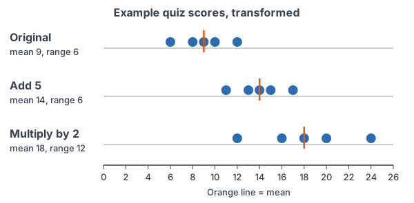
Picture a dot plot of quiz scores. If the teacher adds 5 points to every score, every dot slides 5 to the right. The middle moves 5, but the dots are just as far apart as before.

Now suppose every score is doubled. Each dot moves to twice its value, so the middle doubles, and the gaps between dots double too. In both cases the shape of the plot (skewed, symmetric, and so on) does not change.

Three dot plots of example quiz scores on one number line from 0 to 26. Original scores 6, 8, 9, 10 and 12 have mean 9 and range 6. After adding 5, the scores 11, 13, 14, 15 and 17 have mean 14 and range 6. After multiplying by 2, the scores 12, 16, 18, 20 and 24 have mean 18 and range 12. — Adding 5 slides the whole data set right without changing its spread; multiplying by 2 stretches it, doubling both the mean and the range.

Rules for transforming data

Change to every value	Center and location (mean, median, quartiles, min, max)	Spread (range, IQR, standard deviation)	Shape
Add or subtract a	Add or subtract a	No change	No change
Multiply or divide by b	Multiply or divide by b	Multiply or divide by \|b\|	No change

For a combined change $y = a + bx$ :

\bar{y} = a + b\bar{x} \qquad s_y = |b| \, s_x \qquad s_y^2 = b^2 s_x^2

Spread is never negative, so it uses the absolute value of b. The variance is multiplied by $b^2$ , because it is the square of the standard deviation.

Transforming data examples

Example 1: Add a constant

Five quiz scores are 6, 8, 9, 10 and 12 (example data). The teacher adds 5 points to every score. Find the mean, median, range and standard deviation before and after.

\bar{x} = \dfrac{6 + 8 + 9 + 10 + 12}{5} = \dfrac{45}{5} = 9

Find the original mean.

\text{Median} = 9, \; \text{range} = 12 - 6 = 6

Middle value; largest minus smallest.

9 + 1 + 0 + 1 + 9 = 20

Squared deviations of −3, −1, 0, 1, 3, added.

s = \sqrt{\dfrac{20}{4}} = \sqrt{5} \approx 2.24

Divide by n − 1 = 4 and take the root (see standard deviation).

\text{New mean} = 9 + 5 = 14, \; \text{new median} = 9 + 5 = 14

Adding 5 shifts every measure of center by 5.

\text{New range} = 6, \; \text{new } s \approx 2.24

Adding 5 does not change the spread.

Check: the new scores 11, 13, 14, 15 and 17 add to 70, and 70 ÷ 5 = 14. Their range is 17 − 11 = 6.

Answer: the mean and median rise from 9 to 14; the range stays 6 and the standard deviation stays about 2.24.

Example 2: Multiply by a constant (change units)

A set of heights has mean 60 inches, median 59 inches, standard deviation 3 inches and IQR 4 inches. Convert to centimeters (1 inch = 2.54 cm).

60 \times 2.54 = 152.4

Multiply the mean by 2.54.

59 \times 2.54 = 149.86

Multiply the median by 2.54.

3 \times 2.54 = 7.62

Multiply the standard deviation by 2.54.

4 \times 2.54 = 10.16

Multiply the IQR by 2.54.

Answer: mean 152.4 cm, median 149.86 cm, standard deviation 7.62 cm, IQR 10.16 cm. Every measure, center and spread, is multiplied by 2.54.

Example 3: Celsius to Fahrenheit (word problem)

Daily high temperatures in a city have mean 20 °C and standard deviation 5 °C (example data). Use $F = 32 + 1.8C$ to find the mean, standard deviation and variance in °F.

\bar{F} = 32 + 1.8(20)

Use mean of y = a + b × mean of x, with a = 32 and b = 1.8.

\bar{F} = 32 + 36 = 68

Multiply, then add.

s_F = 1.8 \times 5 = 9

The added 32 does not affect spread; multiply by 1.8.

s_F^2 = 9^2 = 81

Square the standard deviation to get the variance.

Answer: mean 68 °F, standard deviation 9 °F and variance 81 (°F)². Note that the variance in °C was 25, and 25 × 1.8² = 25 × 3.24 = 81.

Example 4: Two kinds of raises

Workers at a shop earn a mean of $15 per hour with a standard deviation of $2.50. Compare (a) a raise of $1 per hour for everyone with (b) a 10% raise for everyone.

\text{(a) mean} = 15 + 1 = 16, \; s = 2.50

Adding $1 shifts the mean but not the spread.

\text{(b) } 1.10 \times 15 = 16.50

A 10% raise multiplies every wage by 1.10 (see percent change).

1.10 \times 2.50 = 2.75

Multiplying also stretches the spread.

Answer: the $1 raise gives mean $16 with standard deviation $2.50. The 10% raise gives mean $16.50 with standard deviation $2.75, because higher-paid workers get bigger raises, so the wages spread apart.

Example 5: Standardizing gives mean 0 and standard deviation 1

A data set has mean 50 and standard deviation 10. Every value is changed to its z-score, $z = \dfrac{x - 50}{10}$ . Find the mean and standard deviation of the z-scores.

z = \dfrac{x}{10} - \dfrac{50}{10} = 0.1x - 5

Write the z-score as a + bx, with b = 0.1 and a = −5.

\bar{z} = -5 + 0.1(50) = -5 + 5 = 0

Apply the rule for the mean.

s_z = 0.1 \times 10 = 1

Apply the rule for the standard deviation.

Answer: the z-scores have mean 0 and standard deviation 1. This is why z-scores let you compare values from different data sets.

Common mistakes

Mistake	Example of the error	Fix
Adding the constant to the spread	Saying the standard deviation becomes 2.24 + 5 after adding 5	Adding a constant never changes the range, IQR or standard deviation.
Multiplying the variance by b	New variance = 1.8 × 25 = 45	Multiply the variance by b²: 25 × 3.24 = 81.
Using a negative factor for spread	With y = 10 − 2x and s = 1.5, saying the new standard deviation is −3	Use \|b\|: 2 × 1.5 = 3.
Adding before multiplying in y = a + bx	Mean of 32 + 1.8C as (20 + 32) × 1.8	Multiply by b first, then add a: 32 + 1.8 × 20 = 68.
Thinking the shape changes	“Doubling makes the data more skewed.”	Adding and multiplying by a positive number keep the same shape.
Expecting percentiles to change	“After adding 5 to everyone, my percentile went up.”	Everyone moved the same way, so each value keeps its percentile.

Related methods

Nonlinear transformations

Taking logs or square roots of every value changes the shape, not just the center and spread. Those transformations straighten curved data in the regression unit. The rules in this lesson apply only to adding and multiplying by constants.

Combining random variables

The same rules hold for random variables: if $Y = a + bX$ , the mean of Y is a + b times the mean of X, and the standard deviation is |b| times that of X. This comes back in the random variables unit.

Practice problems

A data set has mean 12 and standard deviation 3. Every value is increased by 4. Find the new mean and standard deviation.
A data set has mean 12 and standard deviation 3. Every value is multiplied by 5. Find the new mean and standard deviation.
A data set has median 40 and IQR 8. Every value is decreased by 10. Find the new median and IQR.
A data set has mean 7 and standard deviation 2. Find the mean and standard deviation of y = 3x + 1.
A data set has variance 4. Every value is multiplied by 3. What is the new variance?
Heights have mean 5.5 feet and standard deviation 0.25 feet. Convert both to inches (1 foot = 12 inches).
A data set has mean 3 and standard deviation 1.5. Find the mean and standard deviation of y = 10 − 2x.
A data set has minimum 5 and range 20. Every value is doubled, then 3 is added. Find the new minimum and range.
The data 2, 4, 6 have mean 4 and standard deviation 2. Multiply each value by 3 and find the new mean and standard deviation directly.
Test scores have mean 62 and standard deviation 8. The teacher adds 13 points to every score. Find the new mean and standard deviation. Does any student’s percentile change?

Show answers

12 + 4 = 16

Adding 4 shifts the mean by 4.

s = 3

Adding does not change the spread.

Answer: mean 16, standard deviation 3

12 \times 5 = 60

Multiply the mean by 5.

3 \times 5 = 15

Multiply the standard deviation by 5.

Answer: mean 60, standard deviation 15

40 - 10 = 30

Subtracting shifts the median.

\text{IQR} = 8

Subtracting does not change the spread.

Answer: median 30, IQR 8

\bar{y} = 1 + 3(7) = 1 + 21 = 22

Multiply the mean by 3, then add 1.

s_y = 3 \times 2 = 6

Multiply the standard deviation by 3; the +1 has no effect.

Answer: mean 22, standard deviation 6

4 \times 3^2 = 4 \times 9 = 36

Multiply the variance by the square of the factor.

Answer: 36

5.5 \times 12 = 66

Multiply the mean by 12.

0.25 \times 12 = 3

Multiply the standard deviation by 12.

Answer: mean 66 inches, standard deviation 3 inches

\bar{y} = 10 - 2(3) = 10 - 6 = 4

Use a = 10 and b = −2.

s_y = |-2| \times 1.5 = 2 \times 1.5 = 3

Use the absolute value of b (see absolute value).

Answer: mean 4, standard deviation 3

2(5) + 3 = 13

The minimum is a location measure: double it, then add 3.

2 \times 20 = 40

The range is a spread measure: double it; adding 3 has no effect.

Answer: minimum 13, range 40

6, 12, 18 \Rightarrow \bar{y} = \dfrac{36}{3} = 12

Multiply each value by 3, then find the mean.

(-6)^2 + 0^2 + 6^2 = 72

Squared deviations from 12, added.

s_y = \sqrt{\dfrac{72}{2}} = \sqrt{36} = 6

Divide by n − 1 = 2 and take the root.

Answer: mean 12 and standard deviation 6, which match 3 × 4 and 3 × 2

10.

62 + 13 = 75

Adding 13 shifts the mean.

s = 8

The spread does not change.

\text{Order of scores unchanged}

Every score rose by the same amount.

Answer: mean 75, standard deviation 8; no student’s percentile changes

Transforming data FAQ

What happens to the standard deviation when you add a constant?

Nothing. Adding or subtracting the same number moves every value the same distance, so the distances between values, and the standard deviation, stay the same.

What happens to the mean when you multiply every value by a constant?

The mean is multiplied by the same constant. The median, quartiles and standard deviation are multiplied by it too.

How does the variance change when data are multiplied by b?

The variance is multiplied by b². For example, multiplying every value by 3 multiplies the variance by 9.

Does transforming data change the shape of a distribution?

Adding a constant or multiplying by a positive constant keeps the same shape. Multiplying by a negative number flips the distribution, so a right skew becomes a left skew.

Summary

Adding or subtracting a constant shifts the center and location measures by that constant; spread and shape do not change.
Multiplying or dividing by b multiplies or divides the center and location measures by b and the spread by |b|.
For $y = a + bx$ : $\bar{y} = a + b\bar{x}$ and $s_y = |b| s_x$ ; the variance is multiplied by $b^2$ .
Standardizing to z-scores gives mean 0 and standard deviation 1.

Previous lesson: Percentiles and Z-Scores

Next lesson: Comparing Distributions

Back to the Statistics Index