Transformations to Achieve Linearity

A transformation to achieve linearity changes curved data so that it follows a straight line. You take the logarithm, square root or another function of x, y or both. Then you fit a least-squares line to the new values and undo the transformation to make predictions in the original units.

Before this lesson: Least-Squares Regression Line, Residuals and Residual Plots and Logarithms

Why transform curved data

A least-squares line only works well when the data are linear. If the scatter plot bends, or the residual plot shows a curve, a line will predict badly in some places. You could give up on lines, but there is a trick.

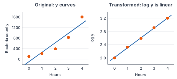
Change the scale of one or both variables. If y grows by the same factor each time x goes up by 1, then log y grows by the same amount each time. That turns the curve into a line. Now all the line tools work again: slope, residuals and $r^2$ .

Two scatter plots of the same data: hours x from 0 to 4 and bacteria count y of 100, 210, 390, 820 and 1600. Left: y against x curves upward, and the straight line y-hat = −98 + 361x misses the pattern. Right: log y against x gives 2.000, 2.322, 2.591, 2.914 and 3.204, which lie almost exactly on the line log y-hat = 2.006 + 0.300x. — Taking the log of y turns exponential growth into a straight line.

Which transformation to use

Pattern in the data	Transform	Linear model	Model in original units
Exponential: y grows by a constant factor	log y against x	$\log \hat{y} = a + bx$	$\hat{y} = 10^{a + bx}$
Power: y grows like a power of x	log y against log x	$\log \hat{y} = a + b \log x$	$\hat{y} = 10^a x^b$
Squared: y grows like $x^2$	$\sqrt{y}$ against x	$\sqrt{\hat{y}} = a + bx$	$\hat{y} = (a + bx)^2$

You can use the natural log, ln, instead of log base 10. Just undo it with $e^x$ instead of $10^x$ .

Steps

Make a scatter plot and a residual plot of the original data. Look for a curve.
Pick a transformation from the table and compute the new values.
Make a scatter plot of the new values. If it looks straight, find the least-squares line.
Check the new residual plot. No pattern means the transformation worked.
To predict, put x into the line, then undo the transformation.

Transformation examples

Example 1: Square root for braking distance

A driving guide lists braking distance y (feet) for speeds x of 20, 30, 40, 50, 60 and 70 mph (example data): 20, 45, 80, 125, 180 and 245 feet. The residual plot for a straight line is U-shaped. Transform with $\sqrt{y}$ and predict the braking distance at 45 mph.

\sqrt{y}: \; 4.47, 6.71, 8.94, 11.18, 13.42, 15.65

Take the square root of each y (see square roots).

6.71 - 4.47 \approx 2.24

Each 10 mph adds about 2.24 to the square root, so the new points lie on a line.

\sqrt{\hat{y}} = 0.2236x

LinReg on x and the square roots gives a ≈ 0 and b ≈ 0.2236, with r = 1.

\sqrt{\hat{y}} = 0.2236(45)

Substitute x = 45.

\sqrt{\hat{y}} \approx 10.062

Multiply.

\hat{y} \approx 10.062^2 \approx 101.2

Square both sides to undo the square root.

Answer: the predicted braking distance at 45 mph is about 101 feet. The model in original units is $\hat{y} = (0.2236x)^2$ , a curve that matches the data.

Example 2: Log of y for exponential growth

A lab counts bacteria every hour (example data): x = 0, 1, 2, 3, 4 hours and y = 100, 210, 390, 820, 1600 bacteria. Fit an exponential model with a log transformation and predict the count at 5 hours.

\log y: \; 2.000, 2.322, 2.591, 2.914, 3.204

Take the log of each y (see logarithms). On a TI-84, set L3 = log(L2).

\log \hat{y} = 2.006 + 0.300x

Run LinReg(a+bx) on L1 and L3. Here r ≈ 0.9997.

\log \hat{y} = 2.006 + 0.300(5)

Substitute x = 5.

\log \hat{y} = 3.506

Multiply, then add.

\hat{y} = 10^{3.506}

Undo the log: raise 10 to both sides.

\hat{y} \approx 3206

Use a calculator.

Answer: about 3,206 bacteria at 5 hours. The model is $\hat{y} = 10^{2.006 + 0.300x}$ . Since $10^{0.3} \approx 2$ , the count roughly doubles every hour.

Example 3: Undo a natural log

A biologist models the number of fruit flies y (hundreds) after x days with $\ln \hat{y} = 1.2 + 0.4x$ (example data). Predict y after 3 days.

\ln \hat{y} = 1.2 + 0.4(3)

Substitute x = 3.

\ln \hat{y} = 1.2 + 1.2 = 2.4

Multiply, then add.

\hat{y} = e^{2.4}

Undo the natural log: raise e to both sides (see the number e).

\hat{y} \approx 11.02

Use a calculator.

Answer: about 11.02 hundred, or roughly 1,102 fruit flies. Always undo the transformation before you state a prediction.

Example 4: Planets and a power model (word problem)

The table gives each planet’s average distance from the Sun, d (in AU, where Earth’s distance is 1), and the time to orbit the Sun, T (in Earth years). Values are rounded from NASA planetary data.

Planet	d (AU)	T (years)
Mercury	0.387	0.241
Venus	0.723	0.615
Earth	1	1
Mars	1.524	1.881
Jupiter	5.203	11.86
Saturn	9.537	29.46

T bends upward as d grows, but not like an exponential. Use log T against log d to predict the orbit time of Uranus, which is 19.19 AU from the Sun.

\log \hat{T} = 0.000 + 1.500 \log d

Take the log of both lists and run LinReg. Here r ≈ 1.0000.

\log \hat{T} = 1.500 \log 19.19

Substitute d = 19.19.

\log \hat{T} \approx 1.500(1.2831)

Find log 19.19.

\log \hat{T} \approx 1.9246

Multiply.

\hat{T} = 10^{1.9246} \approx 84.1

Undo the log: raise 10 to both sides.

Answer: about 84 years, which matches Uranus’s real orbit time. The model is $\hat{T} = d^{1.5}$ , a form of Kepler’s third law: the square of the orbit time equals the cube of the distance.

Example 5: Choose the better model

Use the bacteria data from Example 2. A straight line on the original data gives $\hat{y} = -98 + 361x$ with residuals 198, −53, −234, −165 and 254. The log model has residuals (in log units) −0.006, 0.016, −0.015, 0.008 and −0.002. Which model is better?

r \approx 0.935 \Rightarrow r^2 \approx 0.874

Square r for the straight line.

r \approx 0.9997 \Rightarrow r^2 \approx 0.999

Square r for the log model.

198, -53, -234, -165, 254

The straight-line residuals go positive, negative, positive: a U shape.

-0.006, 0.016, -0.015, 0.008, -0.002

The log-model residuals are tiny and show no pattern.

Answer: the log (exponential) model is better. Its residual plot has no pattern, and it explains about 99.9% of the variation in log y. The straight line has a clear curve in its residuals, even with $r^2 \approx 0.874$ .

Common mistakes

Mistake	Example of the error	Fix
Forgetting to undo the transformation	Reporting 3.506 bacteria at 5 hours	Undo the log: $10^{3.506} \approx 3206$ .
Undoing with the wrong base	Using $10^{2.4}$ for a model with ln	Undo ln with $e^x$ and log with $10^x$ .
Using log y for a power model	Fitting log T against d for the planets	A power model needs log of both variables.
Judging only by r	Keeping the straight line because r ≈ 0.935	Compare residual plots. A curve means the model is wrong.
Comparing r² across different y-scales as if they mean the same thing	“The log model explains 99.9% of the variation in y.”	It explains 99.9% of the variation in log y. Say which variable you mean.
Taking logs of zero or negative values	log 0	Logs only work for positive values. Choose another model if the data include 0 or negatives.

Related methods

Exponential regression on a calculator

Many calculators fit $\hat{y} = ab^x$ directly with ExpReg. That is the same idea as Example 2, done in one step. See exponential regression for the calculator steps, and semi-log plots for why exponential data look straight on a log scale.

Shifting and scaling data

Adding a constant or multiplying by a constant, as in transforming data, does not straighten a curve. Those changes keep the shape. Logs, square roots and powers change the shape, which is why they work here. The rules in properties of logarithms explain why log turns powers into multiples.

Practice problems

Data grow by about the same percent each year. Which transformation should you try?
Data seem to follow $y = ax^b$ for some power b. Which transformation should you try?
A model is $\log \hat{y} = 1.5 + 0.2x$ . Predict y when x = 4.
A model is $\ln \hat{y} = 0.8 + 0.5x$ . Predict y when x = 2.
A model is $\sqrt{\hat{y}} = 3 + 0.5x$ . Predict y when x = 6.
A model is $\log \hat{y} = 0.3 + 2\log x$ . Predict y when x = 10.
Write the model in problem 6 in the form $\hat{y} = ax^b$ .
For (1, 3), (2, 9), (3, 27), (4, 81), take the log of y, find the line, and predict y at x = 5.
The original data have $r^2 = 0.87$ and a curved residual plot. The log-transformed data have $r^2 = 0.99$ and no pattern. Which model should you use?
In Example 2, $\log \hat{y} = 2.006 + 0.300x$ . By what factor does the predicted count grow each hour?

Show answers

\text{constant percent growth}

This is exponential growth.

Answer: log y against x

\log y = \log a + b \log x

Taking logs of a power model gives a line in log x.

Answer: log y against log x

\log \hat{y} = 1.5 + 0.2(4) = 2.3

Substitute x = 4, multiply, then add.

\hat{y} = 10^{2.3} \approx 199.5

Undo the log.

Answer: about 199.5

\ln \hat{y} = 0.8 + 0.5(2) = 1.8

Substitute x = 2, multiply, then add.

\hat{y} = e^{1.8} \approx 6.05

Undo the natural log.

Answer: about 6.05

\sqrt{\hat{y}} = 3 + 0.5(6) = 6

Substitute x = 6, multiply, then add.

\hat{y} = 6^2 = 36

Square both sides.

Answer: 36

\log \hat{y} = 0.3 + 2\log 10

Substitute x = 10.

\log \hat{y} = 0.3 + 2(1) = 2.3

Use log 10 = 1.

\hat{y} = 10^{2.3} \approx 199.5

Undo the log.

Answer: about 199.5

\hat{y} = 10^{0.3 + 2\log x}

Undo the log on both sides.

\hat{y} = 10^{0.3} \cdot 10^{2\log x}

Split the power with the exponent rules.

\hat{y} = 10^{0.3} \cdot x^2

Use $10^{2\log x} = x^2$ .

\hat{y} \approx 2.0x^2

Use $10^{0.3} \approx 1.995$ .

Answer: $\hat{y} \approx 2.0x^2$

\log y: \; 0.477, 0.954, 1.431, 1.908

Take the log of each y.

0.954 - 0.477 = 0.477

Each step in x adds 0.477, so the points are on a line.

\log \hat{y} = 0 + 0.477x

The line starts at 0 when x = 0 and has slope 0.477.

\log \hat{y} = 0.477(5) = 2.385

Substitute x = 5.

\hat{y} = 10^{2.385} \approx 243

Undo the log.

Answer: about 243 (the data are $3^x$ , and $3^5 = 243$ )

r^2 = 0.99, \; \text{no pattern}

The transformed model fits better and its residuals look random.

Answer: the log-transformed model

10.

10^{0.300} \approx 1.995

Each extra hour adds 0.300 to log y, so y is multiplied by 10^0.3.

Answer: about 2; the predicted count roughly doubles every hour

Transformations to achieve linearity FAQ

Why do you take the log of data in regression?

A log turns exponential growth into a straight line. That lets you use the least-squares line, then undo the log to make predictions.

How do you know which transformation to use?

Try log y against x for exponential patterns and log y against log x for power patterns. The right one gives a straight scatter plot and a residual plot with no pattern.

How do you undo a log transformation?

Raise 10 to the predicted value if you used log base 10, or raise e to it if you used ln. For example, $\log \hat{y} = 2.3$ gives $\hat{y} = 10^{2.3} \approx 199.5$ .

Is transformations to achieve linearity on the AP Statistics exam?

It was removed from the AP Statistics framework starting with the 2026–27 course, but it is still taught in many college statistics courses and textbooks.

Summary

Transform curved data so it looks linear, then fit a least-squares line to the new values.
Exponential pattern: log y against x. Power pattern: log y against log x.
Check the new scatter plot and residual plot. No pattern means the transformation worked.
To predict, put x into the line, then undo the transformation with $10^x$ , $e^x$ or squaring.
Compare models with residual plots, not just r.

Previous lesson: Influential Points

Next lesson: Sampling Methods

Back to the Statistics Index