
Residuals and Residual Plots
A residual is the actual y-value minus the predicted y-value: y - \hat{y}. It shows how far a data point is above or below the regression line. A residual plot graphs every residual against x. If the plot shows no pattern, a linear model fits the data well.
Before this lesson: Least-Squares Regression Line, Correlation Coefficient and Scatter Plots and Correlation
What a residual means
A regression line gives a predicted value, \hat{y}, for each x. The real data point is usually a little above or below that prediction. The residual measures that miss.
A positive residual means the point is above the line, so the model predicted too low. A negative residual means the point is below the line, so the model predicted too high. A residual of 0 means the point is right on the line.
Each residual has the same units as y. A residual of 12 drinks means the shop sold 12 more drinks than the line predicted.
Residual formula
\text{residual} = y - \hat{y} = \text{actual} - \text{predicted}To find a residual, first put x into the regression line to get \hat{y}. Then subtract \hat{y} from the actual y. Always subtract in this order: actual minus predicted.
What a residual plot shows
A residual plot is a scatter plot with x on the horizontal axis and the residuals on the vertical axis. A horizontal line at 0 stands for the regression line. Here is how to read one:
- No clear pattern (points scattered above and below 0): a linear model is appropriate.
- A curve (such as a U shape): the data are not linear, so a line is the wrong model.
- A fan shape (spread grows as x grows): predictions are less reliable where the spread is large.
- One point far from 0: that point may be an outlier.
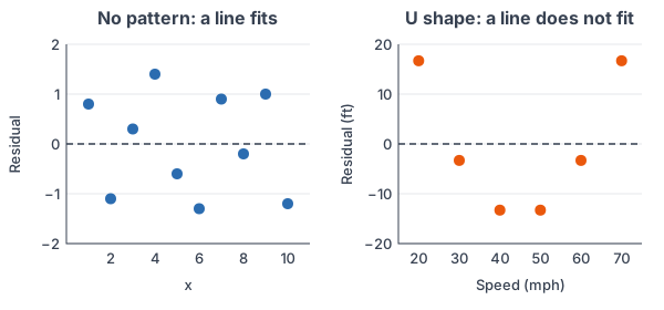
The left plot is what you hope to see. The right plot comes from Example 4 below. Its curve says a straight line misses the shape of the data, even though r for those data is very close to 1.
Residual and residual plot examples
Example 1: Find and interpret one residual
A coffee shop records the daily high temperature x (°F) and the number of iced drinks sold y (example data). The regression line is \hat{y} = -40 + 2.5x. On an 80°F day, the shop sold 172 iced drinks. Find and interpret the residual.
\hat{y} = -40 + 2.5(80)Substitute x = 80 into the line.
\hat{y} = -40 + 200Multiply.
\hat{y} = 160Add.
\text{residual} = 172 - 160Subtract: actual minus predicted.
\text{residual} = 12Simplify.
Answer: the residual is 12. The shop sold 12 more iced drinks than the line predicted for an 80°F day. The point is above the line.
Example 2: Find all the residuals for a data set
A bakery tracks the number of workers on a shift (x) and the dozens of muffins baked (y) (example data): (1, 3), (2, 7), (3, 6), (4, 10), (5, 9). The least-squares regression line is \hat{y} = 2.5 + 1.5x. Find each residual and check that they add to 0.
\hat{y} = 2.5 + 1.5(1) = 4Predict for x = 1.
3 - 4 = -1
Residual for (1, 3): actual minus predicted (see subtracting integers).
\hat{y} = 2.5 + 1.5(2) = 5.5Predict for x = 2.
7 - 5.5 = 1.5
Residual for (2, 7).
\hat{y} = 2.5 + 1.5(3) = 7Predict for x = 3.
6 - 7 = -1
Residual for (3, 6).
\hat{y} = 2.5 + 1.5(4) = 8.5Predict for x = 4.
10 - 8.5 = 1.5
Residual for (4, 10).
\hat{y} = 2.5 + 1.5(5) = 10Predict for x = 5.
9 - 10 = -1
Residual for (5, 9).
-1 + 1.5 - 1 + 1.5 - 1 = 0
Add the residuals to check.
Answer: the residuals are −1, 1.5, −1, 1.5 and −1. They add to 0, as the residuals from a least-squares line always do. The residual plot has the points (1, −1), (2, 1.5), (3, −1), (4, 1.5) and (5, −1).
Example 3: Make a residual plot with a calculator
Use the bakery data from Example 2.
\text{STAT, 1:Edit: } L_1 = \{1, 2, 3, 4, 5\}, \; L_2 = \{3, 7, 6, 10, 9\}Enter x in L1 and y in L2.
\text{STAT, CALC, 8:LinReg(a+bx), ENTER}Run the regression. The TI-84 saves the residuals in a list called RESID.
\text{2nd, Y=, Plot1: Xlist } L_1, \text{ Ylist RESID}Set up a scatter plot. For Ylist, press 2nd, STAT and choose RESID.
\text{ZOOM, 9:ZoomStat}Graph the residual plot.
In Desmos: make a table with columns x_1 and y_1, then type y_1 \sim m x_1 + b. Click “plot” next to the residuals e_1 that Desmos lists under the regression.
Answer: the plot shows the 5 residuals from Example 2, bouncing above and below 0. There is no curve or fan, so a line is a reasonable model. With only 5 points, though, any pattern is hard to judge.
Example 4: Read a residual plot
A driving guide lists braking distance y (feet) for speeds x of 20, 30, 40, 50, 60 and 70 mph (example data): 20, 45, 80, 125, 180 and 245 feet. The regression line is \hat{y} = -86.7 + 4.5x, and r ≈ 0.99. Find the residual at 20 mph, then use the residual plot to judge the line.
\hat{y} = -86.7 + 4.5(20)Substitute x = 20.
\hat{y} = -86.7 + 90 = 3.3Multiply, then add.
\text{residual} = 20 - 3.3 = 16.7Subtract: actual minus predicted.
16.7, -3.3, -13.3, -13.3, -3.3, 16.7
The same steps give all six residuals, in order of speed.
Answer: the residual at 20 mph is 16.7 feet. The residuals go from positive to negative and back to positive, making a U shape (the right plot above). The line is not a good model, even though r ≈ 0.99. Braking distance curves upward as speed grows.
Example 5: Work backward from a residual (word problem)
A real estate model predicts a home’s price y (thousands of dollars) from its size x (square feet): \hat{y} = 50 + 0.12x (example data). A 1,500-square-foot home has a residual of −14. What did it sell for? Did the model overestimate or underestimate its price?
\hat{y} = 50 + 0.12(1500)Substitute x = 1500.
\hat{y} = 50 + 180 = 230Multiply, then add.
y - 230 = -14
Write residual = actual − predicted.
y = -14 + 230
Add 230 to both sides.
y = 216
Simplify.
Answer: the home sold for 216 thousand dollars ($216,000). The residual is negative, so the model overestimated the price by $14,000.
Common mistakes
| Mistake | Example of the error | Fix |
|---|---|---|
| Subtracting in the wrong order | 160 - 172 = -12 for Example 1 | Always use actual minus predicted: 172 - 160 = 12. |
| Mixing up the meaning of the sign | Saying a positive residual means the model predicted too high | Positive: the point is above the line, so the model predicted too low. |
| Graphing y instead of the residuals | Plotting (x, y) and calling it a residual plot | A residual plot puts the residuals, y - \hat{y}, on the vertical axis. |
| Trusting r alone | “r = 0.99, so a line fits the braking data.” | Check the residual plot too. A curve means a line is the wrong model. |
| Calling a fan shape a good fit | Ignoring residuals that spread out as x grows | A fan shape means predictions are less reliable for larger x. |
| Using an old RESID list | Graphing RESID before running LinReg on the new data | Run LinReg(a+bx) first. RESID always holds the last regression. |
Related methods
Standard deviation of the residuals
The standard deviation of the residuals, s, gives the typical size of a prediction error. It works like the standard deviation of a data set, but it divides by n − 2. For the bakery data in Example 2:
s = \sqrt{\dfrac{\sum (y - \hat{y})^2}{n - 2}}\textstyle\sum (y - \hat{y})^2 = 1 + 2.25 + 1 + 2.25 + 1 = 7.5Square each residual and add.
s = \sqrt{\dfrac{7.5}{5 - 2}} = \sqrt{2.5}Divide by n − 2 = 3.
s \approx 1.58
Take the square root (see square roots).
So the line’s predictions are typically off by about 1.58 dozen muffins.
Other ways to judge a line
Start with a scatter plot and the correlation coefficient. Then check the residual plot. The next lesson, Coefficient of Determination, shows how r² measures how much of the variation the line explains. When the residual plot curves, a model like exponential regression may fit better.
Practice problems
- The regression line is \hat{y} = 4 + 2x. Find the residual for the point (3, 12).
- The regression line is \hat{y} = 100 - 3x. Find the residual for the point (10, 65).
- A point has a predicted value of 18.6 and a residual of −2.4. Find its actual y-value.
- For hours studied x and test score y, \hat{y} = 52 + 5x. A student who studied 4 hours has a residual of 6. Find her actual score and interpret the residual.
- The least-squares line for (1, 5), (2, 6), (3, 9), (4, 8) is \hat{y} = 4 + 1.2x. Find all four residuals and check that they add to 0.
- A residual plot for x = 1 to 6 shows the residuals 4, −1, −3, −3, −1, 4. Is a linear model appropriate? Explain.
- A residual plot for x = 1 to 8 shows the residuals 1.2, −0.8, −1.5, 0.9, 0.4, −0.6, 0.3, 0.1. Is a linear model appropriate? Explain.
- In a residual plot, the residuals are close to 0 for small x but spread out farther and farther from 0 as x grows. What does this tell you?
- A line fit to 5 points has residuals 2, −1, −3, 0, 2. Find the standard deviation of the residuals, s.
- A car’s gas use y (gallons) is predicted from miles driven x by \hat{y} = 0.4 + 0.035x. On a 200-mile trip, the car used 6.9 gallons. Find the residual. Did the model overestimate or underestimate?
Show answers
1.
\hat{y} = 4 + 2(3) = 10Substitute x = 3, multiply, then add.
12 - 10 = 2
Subtract: actual minus predicted.
Answer: 2
2.
\hat{y} = 100 - 3(10)Substitute x = 10.
\hat{y} = 100 - 30 = 70Multiply, then subtract.
65 - 70 = -5
Subtract: actual minus predicted.
Answer: −5
3.
y - 18.6 = -2.4
Write residual = actual − predicted.
y = -2.4 + 18.6
Add 18.6 to both sides.
y = 16.2
Simplify.
Answer: 16.2
4.
\hat{y} = 52 + 5(4) = 72Predict for x = 4.
y - 72 = 6
Write residual = actual − predicted.
y = 6 + 72 = 78
Add 72 to both sides.
Answer: 78; she scored 6 points higher than the line predicted
5.
\hat{y} = 5.2, \; 6.4, \; 7.6, \; 8.8Substitute x = 1, 2, 3 and 4 into the line.
5 - 5.2 = -0.2
Residual for (1, 5).
6 - 6.4 = -0.4
Residual for (2, 6).
9 - 7.6 = 1.4
Residual for (3, 9).
8 - 8.8 = -0.8
Residual for (4, 8).
-0.2 - 0.4 + 1.4 - 0.8 = 0
Add the residuals to check.
Answer: −0.2, −0.4, 1.4, −0.8; they add to 0
6.
4, \; -1, \; -3, \; -3, \; -1, \; 4
The residuals go from positive to negative and back to positive.
Answer: no; the residuals make a U-shaped curve, so the data are not linear
7.
1.2, \; -0.8, \; -1.5, \; 0.9, \; 0.4, \; -0.6, \; 0.3, \; 0.1
The signs switch back and forth with no curve or fan.
Answer: yes; the residuals are scattered above and below 0 with no clear pattern
8.
\text{spread of residuals grows with } xThis is a fan shape.
Answer: the line’s predictions are less reliable for larger x, because the errors get bigger there
9.
\textstyle\sum (y - \hat{y})^2 = 4 + 1 + 9 + 0 + 4 = 18Square each residual and add.
s = \sqrt{\dfrac{18}{5 - 2}} = \sqrt{6}Divide by n − 2 = 3.
s \approx 2.45
Take the square root.
Answer: s ≈ 2.45
10.
\hat{y} = 0.4 + 0.035(200)Substitute x = 200.
\hat{y} = 0.4 + 7 = 7.4Multiply, then add.
6.9 - 7.4 = -0.5
Subtract: actual minus predicted.
Answer: −0.5 gallons; the residual is negative, so the model overestimated the gas used
Residuals and residual plots FAQ
How do you calculate a residual?
Put the x-value into the regression line to get the predicted value \hat{y}. Then subtract: residual = actual y − predicted y.
What does a positive residual mean?
The data point is above the regression line. The model predicted a value that was too low.
What does a good residual plot look like?
The points are scattered randomly above and below the zero line, with no curve and no fan shape. That means a linear model is appropriate.
Why do residuals add up to zero?
The least-squares line passes through the middle of the data, so the points above it balance the points below it. For any least-squares line, the residuals add to 0.
Summary
- A residual is actual minus predicted: y - \hat{y}.
- Positive residual: the point is above the line (the model predicted too low). Negative: below the line (too high).
- A residual plot graphs the residuals against x, with a horizontal line at 0.
- No pattern means a line fits. A curve means the data are not linear. A fan means predictions get less reliable.
- The residuals from a least-squares line add to 0, and s gives the typical prediction error.
Previous lesson: Least-Squares Regression Line
Next lesson: Coefficient of Determination
Back to the Statistics Index