
Inference for Regression Slope
Inference for regression slope uses a sample’s slope b to draw conclusions about the true slope β of the population regression line. The test uses t = (b − β₀) ÷ SE_b, and a confidence interval is b ± t* · SE_b, both with df = n − 2. Testing H₀: β = 0 checks for a real linear relationship.
Before this lesson: Least-Squares Regression Line, Residuals and Residual Plots and One-Sample t-Test
Why the slope needs inference
A scatter plot from a sample gives a slope b. A different random sample would give a different line with a different slope. So b is a statistic that varies from sample to sample, just like x̄ or p̂.
The true slope β describes the whole population. If β = 0, knowing x doesn’t help predict y. A test of H₀: β = 0 checks whether the sample slope is too far from 0 to be chance. A confidence interval gives a range of plausible values for β.
The standard error of the slope, SE_b, measures how much b typically varies from sample to sample. Software and calculators report it in the regression output.
Formulas for inference about the slope
t = \dfrac{b - \beta_0}{SE_b}, \qquad b \pm t^* \cdot SE_b, \qquad \text{df} = n - 2SE_b = \dfrac{s}{\sqrt{\sum (x - \bar{x})^2}}, \qquad s = \sqrt{\dfrac{\sum (y - \hat{y})^2}{n - 2}}- b is the sample slope, β₀ is the null value (almost always 0), and n is the number of data points.
- s is the standard deviation of the residuals: the typical distance between a point and the line.
- H₀: β = 0. Hₐ is β > 0, β < 0 or β ≠ 0.
- On a TI-84: put x in L1 and y in L2, then STAT, TESTS, F:LinRegTTest (test) or G:LinRegTInt (interval).
Conditions (LINER)
- Linear: the scatter plot looks linear, and the residual plot shows no curved pattern.
- Independent: when sampling without replacement, n is at most 10% of the population.
- Normal: a histogram or dot plot of the residuals shows no strong skew or outliers.
- Equal SD: the residual plot has about the same spread for all x (no fan shape).
- Random: the data come from a random sample or a randomized experiment.
Inference for regression slope examples
Example 1: Reading regression output
Software output for n = 20 points shows a slope of b = 2.35 with SE_b = 0.82. Find t and df for H₀: β = 0, and the two-sided p-value.
t = \dfrac{2.35 - 0}{0.82} \approx 2.866Subtract β₀ and divide by SE_b.
\text{df} = 20 - 2 = 18Subtract 2 from n.
P(t \ge 2.866) = \text{tcdf}(2.866, 10^{99}, 18) \approx 0.00514Find one tail.
2 \cdot 0.00514 \approx 0.0103
Double it for a two-sided test.
Answer: t ≈ 2.87 with df = 18, and the two-sided p-value is about 0.0103. Software usually prints this two-sided p-value next to the slope.
Example 2: Sleep and reaction speed (word problem)
A researcher records hours of sleep (x) and a reaction-test score (y) for a random sample of 25 adults. The residual plot shows no pattern and the residuals look roughly normal. Software gives b = 0.84 and SE_b = 0.31. Is there convincing evidence that more sleep goes with higher scores? Use α = 0.05.
State: H₀: β = 0 and Hₐ: β > 0, where β is the true slope of the line relating score to hours of sleep for all adults. Plan: t-test for the slope. The LINER conditions are met.
t = \dfrac{0.84 - 0}{0.31} \approx 2.710Subtract β₀ and divide by SE_b.
\text{df} = 25 - 2 = 23Subtract 2 from n.
P(t \ge 2.710) = \text{tcdf}(2.710, 10^{99}, 23)Find the right-tail area.
\approx 0.0063
Read the calculator result.
0.0063 \lt 0.05
Compare the p-value with α.
Conclude: the p-value is about 0.0063, which is less than 0.05, so reject H₀. There is convincing evidence of a positive linear relationship between hours of sleep and reaction score for adults. This is an observational study, so it doesn’t show that sleep causes higher scores.
Example 3: Confidence interval for the slope
Use the output from Example 2 (b = 0.84, SE_b = 0.31, n = 25). Build and interpret a 95% confidence interval for β.
t^* = \text{invT}(0.975, 23) \approx 2.069Find t* for 95% confidence with df = 23.
\text{ME} = 2.069 \cdot 0.31 \approx 0.6414Multiply t* by SE_b.
0.84 - 0.6414 = 0.1986
Subtract ME.
0.84 + 0.6414 = 1.4814
Add ME.
Answer: about (0.199, 1.481). We are 95% confident that each extra hour of sleep goes with an increase of between 0.199 and 1.481 points in the mean reaction score. The interval doesn’t contain 0, which agrees with the test.
Example 4: The test by hand
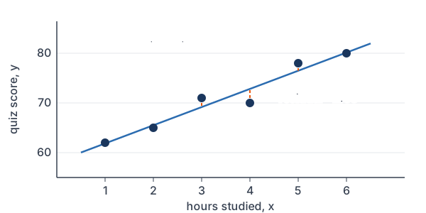
Six randomly chosen students report hours studied (x) and quiz score (y): (1, 62), (2, 65), (3, 71), (4, 70), (5, 78), (6, 80). Test H₀: β = 0 against Hₐ: β > 0 at α = 0.05.
\bar{x} = \dfrac{21}{6} = 3.5Find the mean of x.
\bar{y} = \dfrac{426}{6} = 71Find the mean of y.
6.25 + 2.25 + 0.25 + 0.25 + 2.25 + 6.25 = 17.5
Add the squared x-deviations, Σ(x − x̄)².
22.5 + 9 + 0 + (-0.5) + 10.5 + 22.5 = 64
Add the products (x − x̄)(y − ȳ).
b = \dfrac{64}{17.5} \approx 3.657Divide to get the slope (see least-squares regression line).
a = 71 - 3.657 \cdot 3.5 \approx 58.20
Find the y-intercept, a = ȳ − b·x̄.
The line is ŷ = 58.2 + 3.657x. The table shows each predicted value and residual (see residuals).
| x | 1 | 2 | 3 | 4 | 5 | 6 |
|---|---|---|---|---|---|---|
| y | 62 | 65 | 71 | 70 | 78 | 80 |
| ŷ | 61.86 | 65.51 | 69.17 | 72.83 | 76.49 | 80.14 |
| y − ŷ | 0.14 | −0.51 | 1.83 | −2.83 | 1.51 | −0.14 |
0.14^2 + (-0.51)^2 + 1.83^2 + (-2.83)^2 + 1.51^2 + (-0.14)^2 \approx 13.94
Add the squared residuals.
\dfrac{13.94}{4} = 3.485Divide by n − 2 = 4.
s = \sqrt{3.485} \approx 1.867Take the square root (see square roots).
\sqrt{17.5} \approx 4.183Take the square root of Σ(x − x̄)².
SE_b = \dfrac{1.867}{4.183} \approx 0.4463Divide s by that root.
t = \dfrac{3.657}{0.4463} \approx 8.194Divide b by SE_b.
\text{df} = 6 - 2 = 4Subtract 2 from n.
P(t \ge 8.194) = \text{tcdf}(8.194, 10^{99}, 4) \approx 0.0006Find the right-tail area.
0.0006 \lt 0.05
Compare with α.
Answer: t ≈ 8.19 with df = 4 and a p-value of about 0.0006, so reject H₀. There is convincing evidence of a positive linear relationship between hours studied and quiz score. (With only 6 points, the residuals should be checked carefully for skew or outliers.)
Example 5: Checking conditions with residual plots
Which condition fails in each case? (a) The residual plot shows a clear U-shaped curve. (b) The residual plot fans out, with residuals spreading wider as x grows.
Answer: (a) Linear fails. A curved residual pattern means a line is the wrong model; try a transformation to achieve linearity. (b) Equal SD fails. The spread of y around the line changes with x, so SE_b is not reliable.
Common mistakes
| Mistake | Example of the error | Fix |
|---|---|---|
| Using df = n − 1 | df = 24 for n = 25 | Use df = n − 2 = 23 for slope inference. |
| Using s or s_y for SE_b | t = 0.84/1.9 | Use the slope’s standard error, SE_b, from the output. |
| Interpreting the interval for one person | “Each adult’s score rises 0.199 to 1.481 per hour.” | The slope describes the change in the mean of y. |
| Skipping the residual plot | Running LinRegTTest on curved data | Check LINER first, especially Linear and Equal SD. |
| Claiming cause from observational data | “More sleep causes higher scores.” | Only a randomized experiment supports cause and effect. |
Related methods
Correlation and slope
The slope and the correlation coefficient r always have the same sign, and b = 0 exactly when r = 0. So a test of H₀: β = 0 is also a test of whether the population correlation is 0.
Reading full regression output
Output usually shows the intercept and slope in a “Coef” column, their standard errors in “SE Coef,” and t and p for each. Use the row for the x variable. The output also shows s and r², the coefficient of determination.
Practice problems
- Output for n = 15 gives b = 1.6 and SE_b = 0.5. Find t and df for H₀: β = 0.
- Use Problem 1. Find the two-sided p-value.
- Output for n = 22 gives b = −0.45 and SE_b = 0.12. Build a 95% confidence interval for β.
- How many degrees of freedom does a slope test have with n = 30?
- A study relates hours of screen time (x) to hours of sleep (y). Write H₀ and Hₐ to test whether more screen time goes with less sleep.
- A 95% interval for the slope of price (in dollars) on size (in square feet) is (0.2, 1.5). Interpret it.
- Output for n = 40 gives b = 0.012 and SE_b = 0.009. Test Hₐ: β ≠ 0 at α = 0.05.
- A residual plot spreads out wider as x increases. Which condition fails?
- Why is df = n − 2 for slope inference?
- A 95% interval for β is (−0.3, 0.8). Is there convincing evidence of a linear relationship at α = 0.05?
Show answers
1.
t = \dfrac{1.6 - 0}{0.5} = 3.2Subtract β₀ and divide by SE_b.
\text{df} = 15 - 2 = 13Subtract 2 from n.
Answer: t = 3.2 with df = 13
2.
P(t \ge 3.2) = \text{tcdf}(3.2, 10^{99}, 13) \approx 0.00348Find one tail.
2 \cdot 0.00348 \approx 0.0070
Double it for a two-sided test.
Answer: about 0.0070
3.
\text{df} = 22 - 2 = 20Subtract 2 from n.
t^* = \text{invT}(0.975, 20) \approx 2.086Find t* for 95% confidence.
\text{ME} = 2.086 \cdot 0.12 \approx 0.2503Multiply t* by SE_b.
-0.45 - 0.2503 = -0.7003
Subtract ME.
-0.45 + 0.2503 = -0.1997
Add ME.
Answer: about (−0.700, −0.200)
4.
\text{df} = 30 - 2 = 28Subtract 2 from n.
Answer: df = 28
5.
Answer: H₀: β = 0 and Hₐ: β < 0, where β is the true slope of the line relating sleep to screen time.
6.
Answer: We are 95% confident that each extra square foot goes with an increase of between $0.20 and $1.50 in the mean price.
7.
t = \dfrac{0.012 - 0}{0.009} \approx 1.333Subtract β₀ and divide by SE_b.
\text{df} = 40 - 2 = 38Subtract 2 from n.
P(t \ge 1.333) = \text{tcdf}(1.333, 10^{99}, 38) \approx 0.0952Find one tail.
2 \cdot 0.0952 = 0.1904
Double it for a two-sided test.
0.1904 \gt 0.05
Compare with α.
Answer: p-value ≈ 0.19, so fail to reject H₀. The data don’t give convincing evidence of a linear relationship.
8.
Answer: Equal SD. The spread of the residuals changes with x.
9.
Answer: The line uses two estimates from the data, the slope and the intercept, so 2 degrees of freedom are used up.
10.
Answer: No. The interval contains 0, so β = 0 is plausible, and a two-sided test at α = 0.05 would fail to reject H₀: β = 0.
Inference for regression slope FAQ
How do you test the slope of a regression line?
Use t = (b − 0) ÷ SE_b with df = n − 2, where b and SE_b come from the regression output. A small p-value is evidence that the true slope β is not 0.
How do you find a confidence interval for the slope?
Use b ± t* · SE_b, where t* comes from a t-distribution with df = n − 2. For 95% confidence with n = 25, t* ≈ 2.069.
What are the conditions for inference about a regression slope?
Remember LINER: Linear relationship, Independent observations, Normal residuals, Equal spread of residuals for all x, and Random data.
How do you do a LinRegTTest on a TI-84?
Enter x in L1 and y in L2. Press STAT, choose TESTS, then F:LinRegTTest. Set Xlist and Ylist, choose the direction of Hₐ, then choose Calculate. The screen shows t, p, df, b, s and r².
Summary
- The sample slope b estimates the true slope β, and SE_b measures how much b varies.
- Test: t = (b − β₀) ÷ SE_b. Interval: b ± t* · SE_b. Both use df = n − 2.
- H₀: β = 0 means no linear relationship between x and y.
- Check LINER: Linear, Independent, Normal residuals, Equal SD, Random.
- Interpret the slope as the change in the mean of y for each one-unit increase in x.
Previous lesson: Chi-Square Test for Independence
Next course: Calculus 3 Index
Back to the Statistics Index