Coefficient of Determination (r²): Examples

The coefficient of determination, $r^2$ , is the fraction of the variation in y that a least-squares regression line explains. To find it, square the correlation r, or use $1 - \tfrac{\text{SSE}}{\text{SST}}$ . For example, $r^2 = 0.81$ means the line explains 81% of the variation in y.

Before this lesson: Correlation Coefficient, Least-Squares Regression Line and Residuals and Residual Plots

What r² measures

The y-values in a data set are spread out. Some of that spread happens because x changes, and some is just noise. The coefficient of determination tells you how much of the spread the line accounts for.

Think of two ways to predict y. The first way ignores x and always guesses the mean, $\bar{y}$ . The second way uses the regression line. The value $r^2$ compares how much smaller the errors get when you switch from the mean to the line.

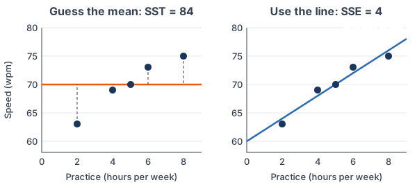
Two scatter plots of the same 5 points: (2, 63), (4, 69), (5, 70), (6, 73) and (8, 75), hours of practice against typing speed. Left: a horizontal line at the mean, y = 70, with dashed gaps −7, −1, 0, 3 and 5; the sum of squared gaps is SST = 84. Right: the regression line y-hat = 60 + 2x with residuals −1, 1, 0, 1 and −1; the sum of squared residuals is SSE = 4. — Using the line shrinks the squared errors from 84 to 4, so r² = 1 − 4/84 ≈ 0.95.

The left graph shows the errors when you guess the mean every time. The right graph shows the much smaller errors when you use the line. These are the data from Example 4.

Coefficient of determination formula

r^2 = 1 - \dfrac{\text{SSE}}{\text{SST}}

Here SSE is the sum of the squared residuals, $\sum (y - \hat{y})^2$ . SST is the total sum of squares, $\sum (y - \bar{y})^2$ , which measures the spread of y around its mean. For a least-squares line, this gives the same number as squaring r:

r^2 = (r)^2

How to interpret r²

Use this sentence, with the names of your variables filled in:

“About __% of the variation in [y] is explained by the linear relationship with [x].”

$r^2$ is always between 0 and 1 (0% to 100%) for a least-squares line.
$r^2$ near 1: the points are close to the line, and the line explains most of the variation.
$r^2$ near 0: the line explains very little. Using x barely beats guessing the mean.
$r^2$ has no sign. To go back to r, take the square root and give it the sign of the slope.

Coefficient of determination examples

Example 1: Find r² from r

For a group of students, hours studied x and test score y have correlation r = 0.9 (example data). Find and interpret $r^2$ .

r^2 = (0.9)^2

Square the correlation.

r^2 = 0.81

Multiply 0.9 by 0.9.

0.81 = 81\%

Change the decimal to a percent (see percentages).

Answer: $r^2 = 0.81$ . About 81% of the variation in test scores is explained by the linear relationship with hours studied. The other 19% comes from other things, such as sleep or past knowledge.

Example 2: Find r² from SSE and SST

A bakery’s data (example data) are (1, 3), (2, 7), (3, 6), (4, 10), (5, 9), with x workers and y dozens of muffins. The line $\hat{y} = 2.5 + 1.5x$ has residuals −1, 1.5, −1, 1.5 and −1. Find $r^2$ .

\bar{y} = \dfrac{35}{5} = 7

Find the mean of y.

y - \bar{y}: \; -4, 0, -1, 3, 2

Subtract 7 from each y.

\text{SST} = 16 + 0 + 1 + 9 + 4 = 30

Square each deviation and add.

\text{SSE} = 1 + 2.25 + 1 + 2.25 + 1 = 7.5

Square each residual and add.

r^2 = 1 - \dfrac{7.5}{30}

Substitute into the formula.

r^2 = 1 - 0.25

Divide.

r^2 = 0.75

Subtract.

Answer: $r^2 = 0.75$ . About 75% of the variation in muffins baked is explained by the linear relationship with the number of workers.

Example 3: Find r from r²

For used cars of one model (example data), age x and price y have $r^2 = 0.64$ . The regression line is $\hat{y} = 30 - 2.5x$ . Find r.

r = \pm\sqrt{0.64}

Undo the square (see square roots).

r = \pm 0.8

Take the square root.

b = -2.5 \rightarrow r \lt 0

The slope is negative, so r is negative.

r = -0.8

Choose the negative root.

Answer: r = −0.8. A common mistake is to stop at 0.8. The sign of r always matches the sign of the slope.

Example 4: Use both formulas and a calculator

Five students record weekly hours of typing practice x and typing speed y (example data): (2, 63), (4, 69), (5, 70), (6, 73), (8, 75). The line is $\hat{y} = 60 + 2x$ , with residuals −1, 1, 0, 1, −1, and r ≈ 0.976. Find $r^2$ two ways, then check with a calculator.

\bar{y} = \dfrac{350}{5} = 70

Find the mean of y.

\text{SST} = 49 + 1 + 0 + 9 + 25 = 84

Square the deviations −7, −1, 0, 3 and 5, then add.

\text{SSE} = 1 + 1 + 0 + 1 + 1 = 4

Square each residual and add.

r^2 = 1 - \dfrac{4}{84} \approx 1 - 0.048

Substitute and divide.

r^2 \approx 0.952

Subtract.

(0.976)^2 \approx 0.953

Check: square r. The tiny difference comes from rounding r.

\text{STAT, CALC, 8:LinReg(a+bx)}

On a TI-84 with DiagnosticOn, the screen shows r² ≈ 0.952.

Answer: $r^2 \approx 0.952$ . About 95% of the variation in typing speed is explained by the linear relationship with practice hours. In Desmos, the regression $y_1 \sim m x_1 + b$ shows the same value as R².

Example 5: Compare two models (word problem)

A utility company wants to predict a home’s monthly energy use. Outdoor temperature has r = −0.85 with energy use, and house size has r = 0.6 (example data). Which variable explains more of the variation in energy use?

(-0.85)^2 = 0.7225

Square r for temperature. A negative times a negative is positive.

0.7225 \approx 72\%

Change to a percent.

(0.6)^2 = 0.36

Square r for house size.

0.36 = 36\%

Change to a percent.

72\% \gt 36\%

Compare.

Answer: temperature. About 72% of the variation in energy use is explained by the linear relationship with temperature, but only 36% by house size. The sign of r doesn’t matter here, because squaring removes it.

Common mistakes

Mistake	Example of the error	Fix
Taking r² as a share of the points	“81% of the points are on the line.”	Say “81% of the variation in y is explained by the linear relationship with x.”
Dropping the sign when finding r	$r^2 = 0.64$ , so r = 0.8, for a line with slope −2.5	Give r the sign of the slope: r = −0.8.
Thinking r² equals r	$r = 0.9$ , so 90% is explained	Square first: $(0.9)^2 = 0.81$ , so 81%.
Trusting a high r² alone	Braking data with $r^2 \approx 0.974$ , so a line fits	Check the residual plot. Those residuals curve, so a line is the wrong model.
Claiming cause and effect	“ $r^2 = 0.9$ , so x causes y.”	r² measures fit, not cause. Only an experiment can show cause and effect.
Swapping SSE and SST	$1 - \tfrac{30}{7.5} = -3$	SSE (residuals) goes on top. For a least-squares line, r² is never negative.

Related methods

r² and the residual plot together

A full check of a linear model uses three tools. Look at the scatter plot, check the residual plot for a pattern, and report $r^2$ and s, the typical size of a residual. A curved residual plot means a line is wrong, even with a high $r^2$ .

Other models

Calculators also report R² for curved models, such as exponential regression. The idea is the same: the share of the variation in y that the model explains.

Practice problems

For a data set, r = 0.7. Find $r^2$ and write it as a percent.
For a data set, r = −0.95. Find $r^2$ .
A regression line has a negative slope, and $r^2 = 0.36$ . Find r.
The regression line is $\hat{y} = 12 + 3x$ , and $r^2 = 0.81$ . Find r.
For a regression, SSE = 12 and SST = 48. Find $r^2$ .
For daily high temperature x and ice cream cones sold y, $r^2 = 0.62$ . Interpret this value in context.
The least-squares line for (1, 5), (2, 6), (3, 9), (4, 8) is $\hat{y} = 4 + 1.2x$ , with residuals −0.2, −0.4, 1.4 and −0.8. Find $r^2$ .
Model A has $r^2 = 0.55$ . Model B has r = −0.8. Which model explains more of the variation in y?
A student says, “Since $r^2 = 0.9$ , more screen time causes lower grades.” Explain the mistake.
A line has $r^2 = 0.98$ , but its residual plot shows a clear U shape. Is the line a good model? Explain.

Show answers

r^2 = (0.7)^2 = 0.49

Square r.

0.49 = 49\%

Change to a percent.

Answer: 0.49, or 49%

r^2 = (-0.95)^2

Square r.

r^2 = 0.9025

A negative times a negative is positive.

Answer: 0.9025 (about 90%)

r = \pm\sqrt{0.36} = \pm 0.6

Take the square root.

r = -0.6

The slope is negative, so r is negative.

Answer: r = −0.6

r = \pm\sqrt{0.81} = \pm 0.9

Take the square root.

r = 0.9

The slope, 3, is positive, so r is positive.

Answer: r = 0.9

r^2 = 1 - \dfrac{12}{48}

Substitute into the formula.

r^2 = 1 - 0.25 = 0.75

Divide, then subtract.

Answer: 0.75

0.62 = 62\%

Change to a percent.

Answer: about 62% of the variation in ice cream cones sold is explained by the linear relationship with daily high temperature

\bar{y} = \dfrac{28}{4} = 7

Find the mean of y.

\text{SST} = 4 + 1 + 4 + 1 = 10

Square the deviations −2, −1, 2 and 1, then add.

\text{SSE} = 0.04 + 0.16 + 1.96 + 0.64 = 2.8

Square each residual and add.

r^2 = 1 - \dfrac{2.8}{10}

Substitute into the formula.

r^2 = 1 - 0.28 = 0.72

Divide, then subtract.

Answer: 0.72

(-0.8)^2 = 0.64

Square r for Model B.

0.64 \gt 0.55

Compare with Model A.

Answer: Model B explains more (64% versus 55%)

r^2 = 0.9

This measures how well the line fits, not why.

Answer: a high r² does not show cause and effect; other variables could explain both, and only a randomized experiment can show causation

10.

r^2 = 0.98

The line explains a lot of the variation.

Answer: no; the U-shaped residual plot shows the data curve, so a curved model would fit better even though r² is high

Coefficient of determination FAQ

What does r² tell you?

It tells you the fraction of the variation in y that the regression line explains. For example, $r^2 = 0.64$ means 64% of the variation in y is explained by the linear relationship with x.

How do you find r² from r?

Square it. If r = −0.7, then $r^2 = (-0.7)^2 = 0.49$ . The result is never negative.

What is a good r² value?

It depends on the field. In physics, values above 0.95 are common, while in social science 0.3 can be useful. A high r² alone never proves a line is the right model, so check the residual plot too.

Is r² the same as r?

No. r gives the direction and strength of a linear relationship and can be negative. $r^2$ is r squared, so it is never negative, and it gives the share of the variation explained.

Summary

The coefficient of determination $r^2$ is the fraction of the variation in y explained by the regression line.
Find it by squaring r, or with $r^2 = 1 - \tfrac{\text{SSE}}{\text{SST}}$ .
Interpret it as “About __% of the variation in y is explained by the linear relationship with x.”
To find r from $r^2$ , take the square root and use the sign of the slope.
A high $r^2$ does not prove a line fits or that x causes y. Check the residual plot.

Previous lesson: Residuals and Residual Plots

Next lesson: Influential Points

Back to the Statistics Index