
Correlation Coefficient
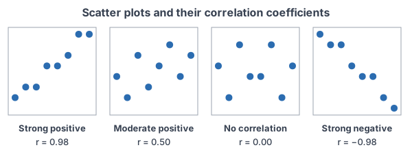
The correlation coefficient, r, measures the direction and strength of a linear relationship between two quantitative variables. It is always between −1 and 1. A positive r means y tends to rise as x rises, and a negative r means y tends to fall. The closer r is to 1 or −1, the closer the points are to a line.
Before this lesson: Scatter Plots and Correlation, Standard Deviation and Percentiles and Z-Scores
What the correlation coefficient measures
A scatter plot shows whether two variables move together. The correlation coefficient puts a number on what you see. Its sign gives the direction (positive or negative), and its size, ignoring the sign, gives the strength: how tightly the points cluster around a straight line.
Think of each point’s z-scores. A point that is above average in both x and y, or below average in both, adds a positive amount to r. A point that is above in one and below in the other adds a negative amount. The correlation coefficient is roughly the average of these products.
Correlation coefficient formula
r = \dfrac{1}{n - 1} \sum \left( \dfrac{x - \bar{x}}{s_x} \right) \left( \dfrac{y - \bar{y}}{s_y} \right)This is the average product of z-scores (dividing by n − 1). The same number comes from a form that is easier by hand:
r = \dfrac{\sum (x - \bar{x})(y - \bar{y})}{\sqrt{\sum (x - \bar{x})^2 \cdot \sum (y - \bar{y})^2}}Properties of r
- r is always between −1 and 1. r = 1 or r = −1 only when every point lies exactly on a line.
- r has no units, and it does not change if you change the units of x or y (for example, hours to minutes).
- Switching x and y gives the same r.
- r measures only linear relationships. A strong curved pattern can have r near 0.
- r is not resistant: one outlier can change it a lot.
- As a rough guide, |r| above 0.8 is strong, 0.5 to 0.8 is moderate, and below 0.5 is weak, but always look at the scatter plot too.
Correlation coefficient examples
Example 1: Find r by hand
Five students record hours studied (x) and quiz score (y) (example data): (1, 62), (2, 68), (3, 74), (4, 72), (5, 84). Find r.
\bar{x} = \dfrac{15}{5} = 3, \; \bar{y} = \dfrac{360}{5} = 72Find both means.
x - \bar{x}: \; -2, -1, 0, 1, 2Subtract 3 from each x.
y - \bar{y}: \; -10, -4, 2, 0, 12Subtract 72 from each y.
\textstyle\sum (x - \bar{x})(y - \bar{y}) = 20 + 4 + 0 + 0 + 24 = 48Multiply each pair of deviations and add.
\textstyle\sum (x - \bar{x})^2 = 4 + 1 + 0 + 1 + 4 = 10Square the x-deviations and add.
\textstyle\sum (y - \bar{y})^2 = 100 + 16 + 4 + 0 + 144 = 264Square the y-deviations and add.
r = \dfrac{48}{\sqrt{10 \cdot 264}} = \dfrac{48}{\sqrt{2640}}Substitute into the formula.
r \approx \dfrac{48}{51.38} \approx 0.934Take the square root and divide (see square roots).
Answer: r ≈ 0.934. There is a strong, positive, linear relationship between hours studied and quiz score for these students.
Example 2: Find r with a calculator
Check Example 1 with technology, and write the interpretation in context.
\text{TI-84: } \text{2nd, 0 (CATALOG), DiagnosticOn, ENTER}Turn on diagnostics once so the calculator shows r.
\text{STAT, 1:Edit: } L_1 = \{1, 2, 3, 4, 5\}, \; L_2 = \{62, 68, 74, 72, 84\}Enter x in L1 and y in L2.
\text{STAT, CALC, 8:LinReg(a+bx)} \Rightarrow r \approx 0.934Run the regression and read r.
In Desmos: type x_1 = [1, 2, 3, 4, 5] and y_1 = [62, 68, 74, 72, 84], then corr(x_1, y_1). Desmos shows 0.934.
Answer: r ≈ 0.934. “There is a strong, positive, linear association between hours studied and quiz score: students who studied more tended to score higher.”
Example 3: Describe several correlations
Describe the direction and strength for each r: (a) 0.91, (b) −0.65, (c) 0.08, (d) −0.97.
\text{(a) } 0.91 \gt 0.8Positive and above 0.8: strong positive.
\text{(b) } |-0.65| = 0.65Negative, between 0.5 and 0.8: moderate negative.
\text{(c) } 0.08 \lt 0.5Very close to 0: very weak or no linear relationship.
\text{(d) } |-0.97| = 0.97Negative and close to 1 in size: very strong negative.
Answer: (a) strong positive, (b) moderate negative, (c) almost no linear relationship, (d) very strong negative. Note that −0.97 is stronger than 0.91; the sign gives direction only.
Example 4: One outlier changes r (word problem)
A coach records weeks of training (x) and the longest run in miles (y) for 6 runners (example data): (2, 4), (3, 5), (4, 7), (5, 8), (6, 9), (7, 11). A 7th runner trained 14 weeks but was injured and ran only 3 miles. How does adding (14, 3) change r?
r \approx 0.994
For the first 6 runners, LinReg or corr( gives r ≈ 0.994: a very strong positive relationship.
\text{Add } (14, 3)Enter the 7th point in L1 and L2 and run the calculation again.
r \approx -0.165
The new r is about −0.165.
Answer: one unusual point changed r from about 0.994 to about −0.165. The correlation coefficient is not resistant, so always graph the data and check for outliers before trusting r.
Example 5: Units and cause
In Example 1, the quiz scores are changed to percents of a 90-point quiz, and the hours to minutes. What is the new r? Does r ≈ 0.934 prove that studying causes higher scores?
\text{minutes} = 60 \times \text{hours}Changing units multiplies every x by a positive number (see transforming data).
\text{percent} = \dfrac{100}{90} \times \text{score}Every y is also multiplied by a positive number.
r = 0.934 \text{ (unchanged)}The z-scores do not change, so r does not change.
Answer: r stays about 0.934. And no, correlation alone does not prove cause and effect: students who study more may also sleep more or attend class more often. Only a randomized experiment can show causation.
Common mistakes
| Mistake | Example of the error | Fix |
|---|---|---|
| Thinking a negative r is weaker | “r = −0.9 is weaker than r = 0.6.” | Strength depends on the size of r. −0.9 is stronger than 0.6. |
| Saying r = 0 means no relationship | A U-shaped scatter plot with r = 0 called “unrelated” | r = 0 means no linear relationship. Look at the graph for curves. |
| Treating correlation as causation | “Shoe size causes better reading.” | A lurking variable (here, age) can explain both. Only experiments show cause. |
| Calculating r for categorical data | Finding r between eye color and favorite sport | r needs two quantitative variables. |
| Trusting r without a graph | Reporting r = −0.165 for Example 4 without noticing the outlier | Always make a scatter plot first. |
| Expecting r over 1 or under −1 | “r = 1.2 shows a very strong link.” | r is always between −1 and 1. Check your arithmetic. |
Related methods
From correlation to a line
When r shows a strong linear relationship, the next step is the least-squares regression line, which predicts y from x. Its slope equals r \cdot \tfrac{s_y}{s_x}, so r connects directly to the line. Later, r² tells what fraction of the variation in y the line explains.
Correlation in earlier courses
The scatter plots and correlation lesson introduces positive, negative and no correlation by looking at a graph, and the line of best fit lesson fits a line by eye.
Practice problems
- Which correlation shows the strongest linear relationship: 0.72, −0.91, 0.05 or −0.4?
- For temperature (x) and home heating cost (y), r = −0.78. Interpret r in context.
- Find r for the points (1, 3), (2, 5), (3, 4).
- Find r for the points (2, 9), (4, 7), (6, 4), (8, 0). Round to three decimal places.
- Heights and weights of students have r = 0.65. What is r if the heights are changed from inches to centimeters?
- A scatter plot has r = 0. Does this mean x and y are unrelated? Explain.
- A student reports r = 1.2. What is wrong?
- For children in grades 1 to 6, shoe size and reading score have r = 0.8. Does a bigger shoe size cause better reading? Explain.
- Every y-value in a data set is multiplied by −1. What happens to r?
- Five points all lie on the line y = 3 − 2x. What is r?
Show answers
1.
|-0.91| = 0.91
Compare sizes: 0.91 is larger than 0.72, 0.4 and 0.05.
Answer: −0.91
2.
r \lt 0, \; |r| = 0.78
Negative direction, moderate to strong strength.
Answer: there is a moderately strong, negative, linear relationship: on warmer days, heating costs tend to be lower
3.
\bar{x} = 2, \; \bar{y} = 4Find the means.
\textstyle\sum (x - \bar{x})(y - \bar{y}) = (-1)(-1) + (0)(1) + (1)(0) = 1Multiply deviations and add.
\textstyle\sum (x - \bar{x})^2 = 2, \; \sum (y - \bar{y})^2 = 2Squared deviations: 1 + 0 + 1 and 1 + 1 + 0.
r = \dfrac{1}{\sqrt{2 \cdot 2}} = \dfrac{1}{2} = 0.5Substitute and simplify.
Answer: r = 0.5
4.
\bar{x} = 5, \; \bar{y} = 5Find the means: 20 ÷ 4 and 20 ÷ 4.
\textstyle\sum (x - \bar{x})(y - \bar{y}) = -12 - 2 - 1 - 15 = -30Products of (−3)(4), (−1)(2), (1)(−1), (3)(−5).
\textstyle\sum (x - \bar{x})^2 = 20, \; \sum (y - \bar{y})^2 = 469 + 1 + 1 + 9 and 16 + 4 + 1 + 25.
r = \dfrac{-30}{\sqrt{920}} \approx \dfrac{-30}{30.33} \approx -0.989Substitute and simplify.
Answer: r ≈ −0.989
5.
\text{Inches to centimeters multiplies } x \text{ by } 2.54A positive change of units does not change z-scores.
Answer: r = 0.65
6.
r = 0 \Rightarrow \text{no linear pattern}r only measures straight-line relationships.
Answer: no; x and y could have a strong curved relationship, so look at the scatter plot
7.
-1 \le r \le 1
r can never be outside this interval.
Answer: r = 1.2 is impossible, so there is a calculation error
8.
\text{Age affects both}Older children have bigger feet and read better.
Answer: no; age is a lurking variable, and correlation does not show causation
9.
\text{Each } y\text{-deviation changes sign}Every product (x − x̄)(y − ȳ) changes sign, but the squares do not.
Answer: r changes sign but keeps its size (for example, 0.6 becomes −0.6)
10.
\text{All points on a line with slope } -2The points fit a line exactly, and the line falls.
Answer: r = −1
Correlation coefficient FAQ
What does the correlation coefficient tell you?
It tells you the direction (positive or negative) and the strength of a linear relationship between two quantitative variables, on a scale from −1 to 1.
What is a strong correlation coefficient?
As a rough guide, an r with size above 0.8 (such as 0.85 or −0.9) is strong, 0.5 to 0.8 is moderate, and below 0.5 is weak. Always check the scatter plot too.
How do you calculate r on a TI-84?
Turn on DiagnosticOn from the CATALOG, enter x in L1 and y in L2, then run STAT, CALC, 8:LinReg(a+bx). The value of r appears with the regression results.
Does correlation mean causation?
No. A strong correlation can come from a lurking variable that affects both variables, or from chance. Only a well-designed experiment can show cause and effect.
Summary
- r measures the direction and strength of a linear relationship and is always between −1 and 1.
- r = \tfrac{1}{n - 1} \sum z_x z_y, or use the deviation form by hand; use LinReg or corr( to check.
- r has no units and does not change when units change or when x and y are switched.
- r measures only linear patterns and is not resistant to outliers, so always graph first.
- Correlation does not imply causation.
Previous lesson: Comparing Distributions
Next lesson: Least-Squares Regression Line
Back to the Statistics Index