Least-Squares Regression Line: Examples

The least-squares regression line is the line that fits a scatter plot best by making the sum of the squared residuals as small as possible. Its equation is $\hat{y} = a + bx$ , where b is the slope and a is the y-intercept. You use it to predict a value of y from a value of x.

Before this lesson: Correlation Coefficient, Line of Best Fit and Slope-Intercept Form

What the least-squares regression line does

A scatter plot with a linear pattern can be summed up by one straight line. Many lines look close, so statistics uses a rule to pick exactly one. The rule is based on residuals.

A residual is the actual y-value minus the predicted y-value: $y - \hat{y}$ . On a graph, it is the vertical gap between a point and the line. Points above the line have positive residuals, and points below have negative ones.

The least-squares line squares every residual and adds them up. It is the one line that makes this total as small as possible. Squaring keeps negative gaps from canceling positive ones, and it punishes big misses more than small ones.

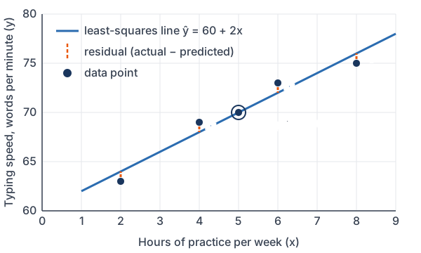
Scatter plot of 5 example points: (2, 63), (4, 69), (5, 70), (6, 73) and (8, 75), with hours of practice from 0 to 9 on the x-axis and typing speed from 60 to 80 words per minute on the y-axis. The line y-hat = 60 + 2x passes through the mean point (5, 70). Dashed vertical segments show the residuals −1, 1, 0, 1 and −1. — The residuals are −1, 1, 0, 1 and −1, so the sum of squared residuals is 4. No other line gives a smaller sum.

The graph uses the data from Example 1 below. The hat on $\hat{y}$ (read “y-hat”) means “predicted y.” The line gives predictions, not the actual data values.

Least-squares regression line formula

\hat{y} = a + bx

Find the slope b first, then the y-intercept a. With summary statistics, use the correlation r and the standard deviations:

b = r \cdot \dfrac{s_y}{s_x} \qquad a = \bar{y} - b\bar{x}

With raw data, the slope comes from the deviations, the same sums used to find r:

b = \dfrac{\sum (x - \bar{x})(y - \bar{y})}{\sum (x - \bar{x})^2}

Properties of the least-squares line

The line always passes through the point $(\bar{x}, \bar{y})$ .
The slope b always has the same sign as r.
The residuals always add up to 0.
The slope b is the predicted change in y when x goes up by 1.
The y-intercept a is the predicted y when x = 0. It only has meaning if x = 0 makes sense for the data.
Predicting x from y gives a different line. Always put the explanatory variable (the one you predict from) on the x-axis.

Least-squares regression line examples

Example 1: Find the line by hand

Five students record weekly hours of typing practice (x) and typing speed in words per minute (y) (example data): (2, 63), (4, 69), (5, 70), (6, 73), (8, 75). Find the least-squares regression line.

\bar{x} = \dfrac{25}{5} = 5, \; \bar{y} = \dfrac{350}{5} = 70

Find both means.

x - \bar{x}: \; -3, -1, 0, 1, 3

Subtract 5 from each x.

y - \bar{y}: \; -7, -1, 0, 3, 5

Subtract 70 from each y.

\textstyle\sum (x - \bar{x})(y - \bar{y}) = 21 + 1 + 0 + 3 + 15 = 40

Multiply each pair of deviations and add.

\textstyle\sum (x - \bar{x})^2 = 9 + 1 + 0 + 1 + 9 = 20

Square the x-deviations and add.

b = \dfrac{40}{20} = 2

Divide to find the slope.

a = 70 - 2(5)

Substitute into a = ȳ − bx̄.

a = 70 - 10 = 60

Multiply, then subtract.

\hat{y} = 60 + 2x

Write the equation (see slope-intercept form).

Answer: $\hat{y} = 60 + 2x$ . For each extra hour of practice per week, the predicted typing speed goes up by 2 words per minute. A student who practices 0 hours has a predicted speed of 60 words per minute.

Example 2: Find the line with a calculator

Check Example 1 with technology.

\text{STAT, 1:Edit: } L_1 = \{2, 4, 5, 6, 8\}, \; L_2 = \{63, 69, 70, 73, 75\}

Enter x in L1 and y in L2.

\text{STAT, CALC, 8:LinReg(a+bx), ENTER}

Run the regression on L1 and L2.

a = 60, \; b = 2, \; r \approx 0.976

Read a, b and r (r shows only when DiagnosticOn is set).

In Desmos: make a table with columns $x_1$ and $y_1$ , then type $y_1 \sim m x_1 + b$ . Desmos shows m = 2 and b = 60. Notice that Desmos uses m for the slope and b for the intercept.

Answer: the calculator gives the same line, $\hat{y} = 60 + 2x$ , with r ≈ 0.976.

Example 3: Use summary statistics

For a sample of adult men (example data), height x has mean 68 inches and standard deviation 3 inches. Weight y has mean 160 pounds and standard deviation 24 pounds, and r = 0.6. Find the regression line and predict the weight of a man 70 inches tall.

b = 0.6 \cdot \dfrac{24}{3}

Substitute into b = r · sy/sx (see correlation coefficient).

b = 0.6 \cdot 8

Divide 24 by 3.

b = 4.8

Multiply.

a = 160 - 4.8(68)

Substitute into a = ȳ − bx̄.

a = 160 - 326.4 = -166.4

Multiply, then subtract.

\hat{y} = -166.4 + 4.8x

Write the equation.

\hat{y} = -166.4 + 4.8(70)

Substitute x = 70.

\hat{y} = -166.4 + 336 = 169.6

Multiply, then add.

Answer: $\hat{y} = -166.4 + 4.8x$ , and the predicted weight is 169.6 pounds. Each extra inch of height predicts 4.8 more pounds, on average. The intercept has no real meaning, because no adult is 0 inches tall.

Example 4: Predictions, residuals and extrapolation

Use the line from Example 1. (a) Predict the speed for 3 hours of practice. (b) Find the residual for the student at (6, 73). (c) Should you use the line to predict the speed for 40 hours?

\hat{y} = 60 + 2(3)

(a) Substitute x = 3.

\hat{y} = 60 + 6 = 66

Multiply, then add.

\hat{y} = 60 + 2(6) = 72

(b) Predict for x = 6.

\text{residual} = 73 - 72 = 1

Subtract: actual minus predicted.

\hat{y} = 60 + 2(40) = 140

40 \gt 8

40 hours is far outside the data, which run from 2 to 8 hours.

Answer: (a) 66 words per minute. (b) The residual is 1, so this student types 1 word per minute faster than predicted. (c) No. Predicting far outside the range of the x-data is called extrapolation, and 140 words per minute is not believable.

Example 5: Used-car prices (word problem)

A used-car lot lists five cars of the same model (example data). Age x is in years, and price y is in thousands of dollars: (1, 28), (2, 24), (4, 21), (5, 17), (8, 10). Find the least-squares regression line, interpret the slope, and predict the price of a 3-year-old car.

\bar{x} = \dfrac{20}{5} = 4, \; \bar{y} = \dfrac{100}{5} = 20

Find both means.

x - \bar{x}: \; -3, -2, 0, 1, 4

Subtract 4 from each x.

y - \bar{y}: \; 8, 4, 1, -3, -10

Subtract 20 from each y.

\textstyle\sum (x - \bar{x})(y - \bar{y}) = -24 - 8 + 0 - 3 - 40 = -75

Multiply each pair of deviations and add (see multiplying integers).

\textstyle\sum (x - \bar{x})^2 = 9 + 4 + 0 + 1 + 16 = 30

Square the x-deviations and add.

b = \dfrac{-75}{30} = -2.5

Divide to find the slope.

a = 20 - (-2.5)(4)

Substitute into a = ȳ − bx̄.

a = 20 + 10 = 30

Multiply, then add.

\hat{y} = 30 - 2.5x

Write the equation.

\hat{y} = 30 - 2.5(3)

Substitute x = 3.

\hat{y} = 30 - 7.5 = 22.5

Multiply, then subtract.

Answer: $\hat{y} = 30 - 2.5x$ . For each extra year of age, the predicted price drops by 2.5 thousand dollars ($2,500). A 3-year-old car has a predicted price of 22.5 thousand dollars, or $22,500.

Common mistakes

Mistake	Example of the error	Fix
Switching x and y	Predicting typing speed with a line that regresses hours on speed	Put the variable you predict from on the x-axis. The two lines are different.
Leaving out “predicted”	“Each hour of practice raises speed by 2 words per minute.”	Say “the predicted speed increases by 2 words per minute” or “on average.”
Flipping the slope formula	$b = r \cdot \tfrac{s_x}{s_y}$	Use $b = r \cdot \tfrac{s_y}{s_x}$ : the spread of y goes on top.
Extrapolating	Predicting 140 words per minute for 40 hours of practice	Only predict inside the range of the x-data.
Mixing up letters in Desmos	Reading Desmos’s b = 60 as the slope	In $\hat{y} = a + bx$ , b is the slope. Desmos’s $y \sim mx + b$ uses m for the slope.
Writing y instead of $\hat{y}$	$y = 60 + 2x$	Write $\hat{y}$ , because the line gives predicted values.

Related methods

By eye versus least squares

The line of best fit lesson draws a line by eye, so two people can get two different lines. The least-squares rule always gives the same line for the same data. Both start with a scatter plot.

Curved data

A straight line only makes sense when the scatter plot is roughly linear. When the data curve, try exponential regression or straighten the data with a transformation, a topic later in this unit.

Checking the fit

Residuals tell you whether a line is a good model. The next lesson, Residuals and Residual Plots, graphs them to check for patterns.

Practice problems

The regression line is $\hat{y} = 12 + 3.5x$ . Predict y when x = 4.
A regression line has slope b = 4. The means are $\bar{x} = 10$ and $\bar{y} = 50$ . Find the y-intercept a and write the line.
For a data set, r = 0.8, $s_x = 2$ , $s_y = 5$ , $\bar{x} = 6$ and $\bar{y} = 20$ . Find the least-squares regression line.
Find the least-squares regression line for the points (1, 2), (2, 4), (3, 3), (4, 7).
For hours studied (x) and test score (y), $\hat{y} = 58 + 4.2x$ . Interpret the slope.
For adults, height x in centimeters and weight y in kilograms give $\hat{y} = -95 + 0.95x$ . Does the y-intercept have a useful meaning? Explain.
The car line from Example 5, $\hat{y} = 30 - 2.5x$ , came from cars 1 to 8 years old. Predict the price of a 15-year-old car and comment.
For a data set, r = −0.6, $s_x = 4$ and $s_y = 10$ . Find the slope b.
A least-squares regression line is $\hat{y} = 8 + 2x$ , and $\bar{x} = 6$ . Find $\bar{y}$ .
In problem 3, suppose you predict x from y instead. Is the new slope $\tfrac{1}{2}$ , the reciprocal of the old slope? Explain.

Show answers

\hat{y} = 12 + 3.5(4)

Substitute x = 4.

\hat{y} = 12 + 14 = 26

Multiply, then add.

Answer: 26

a = 50 - 4(10)

Substitute into a = ȳ − bx̄.

a = 50 - 40 = 10

Multiply, then subtract.

Answer: a = 10, so $\hat{y} = 10 + 4x$

b = 0.8 \cdot \dfrac{5}{2}

Substitute into b = r · sy/sx.

b = 0.8 \cdot 2.5

Divide 5 by 2.

b = 2

Multiply.

a = 20 - 2(6)

Substitute into a = ȳ − bx̄.

a = 20 - 12 = 8

Multiply, then subtract.

Answer: $\hat{y} = 8 + 2x$

\bar{x} = \dfrac{10}{4} = 2.5, \; \bar{y} = \dfrac{16}{4} = 4

Find both means.

x - \bar{x}: \; -1.5, -0.5, 0.5, 1.5

Subtract 2.5 from each x.

y - \bar{y}: \; -2, 0, -1, 3

Subtract 4 from each y.

\textstyle\sum (x - \bar{x})(y - \bar{y}) = 3 + 0 - 0.5 + 4.5 = 7

Multiply each pair of deviations and add.

\textstyle\sum (x - \bar{x})^2 = 2.25 + 0.25 + 0.25 + 2.25 = 5

Square the x-deviations and add.

b = \dfrac{7}{5} = 1.4

Divide to find the slope.

a = 4 - 1.4(2.5)

Substitute into a = ȳ − bx̄.

a = 4 - 3.5 = 0.5

Multiply, then subtract.

Answer: $\hat{y} = 0.5 + 1.4x$

b = 4.2

The slope is the predicted change in y for each 1-unit increase in x.

Answer: for each additional hour studied, the predicted test score goes up by 4.2 points

\hat{y} = -95 + 0.95(0) = -95

The intercept is the prediction when x = 0.

x = 0 \text{ cm}

No adult is 0 cm tall, so x = 0 is far outside the data.

Answer: no; a weight of −95 kg is impossible, and the intercept only places the line

\hat{y} = 30 - 2.5(15)

Substitute x = 15.

\hat{y} = 30 - 37.5 = -7.5

Multiply, then subtract.

15 \gt 8

15 years is outside the data, which run from 1 to 8 years.

Answer: −7.5 thousand dollars, which is impossible; this is extrapolation, so the line should not be used here

b = -0.6 \cdot \dfrac{10}{4}

Substitute into b = r · sy/sx.

b = -0.6 \cdot 2.5

Divide 10 by 4.

b = -1.5

Multiply.

Answer: b = −1.5

\bar{y} = 8 + 2(6)

The line passes through (x̄, ȳ), so substitute x̄ = 6.

\bar{y} = 8 + 12 = 20

Multiply, then add.

Answer: $\bar{y} = 20$

10.

\text{new slope} = r \cdot \dfrac{s_x}{s_y}

Now x is predicted, so the spread of x goes on top.

\text{new slope} = 0.8 \cdot \dfrac{2}{5}

Substitute r = 0.8, sx = 2 and sy = 5.

\text{new slope} = 0.8 \cdot 0.4

Divide 2 by 5.

\text{new slope} = 0.32

Multiply.

\dfrac{1}{b} = \dfrac{1}{2} = 0.5

Find the reciprocal of the old slope, b = 2.

Answer: no; the new slope is 0.32, not 0.5. The two regression lines are different unless r = 1 or r = −1

Least-squares regression line FAQ

What is the least-squares regression line?

It is the straight line $\hat{y} = a + bx$ that makes the sum of the squared residuals as small as possible. It is the standard line used to predict y from x.

How do you find the least-squares regression line on a TI-84?

Enter x in L1 and y in L2, then choose STAT, CALC, 8:LinReg(a+bx) and press ENTER. The screen shows a (the y-intercept) and b (the slope).

What does the slope of a regression line mean?

The slope is the predicted change in y for each 1-unit increase in x. For example, a slope of 2.5 means y is predicted to rise 2.5 units, on average, for every unit of x.

Why is it called “least squares”?

Each residual is squared, and the squares are added. The least-squares line is the line with the least (smallest) possible total.

Summary

The least-squares regression line $\hat{y} = a + bx$ minimizes the sum of the squared residuals.
Slope: $b = r \cdot \tfrac{s_y}{s_x}$ ; intercept: $a = \bar{y} - b\bar{x}$ . Check with LinReg(a+bx).
The line passes through $(\bar{x}, \bar{y})$ , and b has the same sign as r.
Interpret b as the predicted change in y per 1 unit of x, and a only when x = 0 makes sense.
A residual is $y - \hat{y}$ . Avoid extrapolation outside the range of the x-data.

Previous lesson: Correlation Coefficient

Next lesson: Residuals and Residual Plots

Back to the Statistics Index