
Influential Points
An influential point is a data point that changes the least-squares regression line a lot when you remove it. Points with x-values far from the rest, called high-leverage points, are often influential. An outlier in regression is a point with a large residual. To check influence, find the line with and without the point.
Before this lesson: Least-Squares Regression Line, Residuals and Residual Plots and Coefficient of Determination
Outliers, high leverage and influence
Most points in a scatter plot follow the overall pattern. A few points stand apart, and they can stand apart in different ways. Statistics uses three words for them.
- Outlier: a point far above or below the line, so its residual is large. It breaks the y-pattern.
- High-leverage point: a point whose x-value is much smaller or much larger than the other x-values.
- Influential point: a point that changes the slope, the y-intercept or the correlation a lot when you remove it.
Think of the regression line as a seesaw balanced at (\bar{x}, \bar{y}). A point near the middle of the x-values can’t tip it much. A point far out on the end has a long lever arm, so it can tip the line a lot. That is why high-leverage points are often influential.
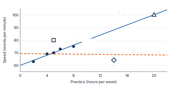
Examples 1 to 3 below add each of these points to the typing data, one at a time.
How to tell if a point is influential
- Look at the x-value. Is it far from the other x-values? Then the point has high leverage.
- Find the residual. Is it large compared with the others? Then the point is an outlier.
- Find the regression line with the point and without it. If the slope, the y-intercept or r changes a lot, the point is influential.
There is no fixed cutoff for “a lot.” Compare the two lines in context and ask whether your conclusions would change.
Influential point examples
Examples 1 to 3 start with the typing data from the least-squares regression line lesson: (2, 63), (4, 69), (5, 70), (6, 73), (8, 75), with hours of practice x and words per minute y (example data). Their line is \hat{y} = 60 + 2x, with r ≈ 0.976.
Example 1: An outlier in the middle
Add the point A = (5, 80). Classify it and find the new line.
\hat{y} = 60 + 2(5) = 70Predict for x = 5 with the original line.
80 - 70 = 10
Find the residual. The others are all between −1 and 1.
\bar{x} = \dfrac{30}{6} = 5Find the new mean of x. It is still 5.
5 - \bar{x} = 0Point A’s x-deviation is 0, so it adds 0 to both sums for the slope.
b = \dfrac{40}{20} = 2The slope stays the same.
\bar{y} = \dfrac{430}{6} \approx 71.67Find the new mean of y.
a = 71.67 - 2(5) = 61.67
Substitute into a = ȳ − bx̄.
Answer: A is an outlier (residual 10), but it does not have high leverage. The new line is \hat{y} = 61.67 + 2x, so the slope stays 2 and the line just moves up. A calculator shows r drops from 0.976 to about 0.691, so the outlier weakens the correlation a lot.
Example 2: High leverage, but not influential
Add the point B = (20, 100) to the original five points. Classify it.
\bar{x} = \dfrac{45}{6} = 7.5Find the new mean of x.
20 - 7.5 = 12.5
B is 12.5 hours from the mean. The other x-values run from 2 to 8.
\hat{y} = 60 + 2(20) = 100Predict for x = 20 with the original line.
100 - 100 = 0
Find the residual. B sits right on the line.
\text{LinReg: } a = 60, \; b = 2, \; r \approx 0.998Run the regression on all 6 points.
Answer: B has high leverage, but it is not influential. The line stays \hat{y} = 60 + 2x, because B follows the same pattern. It does make r stronger, from 0.976 to 0.998.
Example 3: An influential point
Add the point C = (14, 64) to the original five points. Find the new line and compare.
\bar{x} = \dfrac{39}{6} = 6.5, \; \bar{y} = \dfrac{414}{6} = 69Find both new means.
x - \bar{x}: \; -4.5, -2.5, -1.5, -0.5, 1.5, 7.5Subtract 6.5 from each x.
y - \bar{y}: \; -6, 0, 1, 4, 6, -5Subtract 69 from each y.
\textstyle\sum (x - \bar{x})(y - \bar{y}) = 27 + 0 - 1.5 - 2 + 9 - 37.5 = -5Multiply each pair and add (see multiplying integers).
\textstyle\sum (x - \bar{x})^2 = 20.25 + 6.25 + 2.25 + 0.25 + 2.25 + 56.25 = 87.5Square the x-deviations and add.
b = \dfrac{-5}{87.5} \approx -0.057Divide to find the slope.
a = 69 - (-0.057)(6.5) \approx 69.37
Substitute into a = ȳ − bx̄, multiply, then add.
Answer: the new line is \hat{y} = 69.37 - 0.057x. One point changed the slope from 2 to about −0.06, and r goes from 0.976 to about −0.05. Point C is high leverage and very influential.
Example 4: Check influence with a calculator
Use a TI-84 to compare the typing data with and without point C.
L_1 = \{2, 4, 5, 6, 8, 14\}, \; L_2 = \{63, 69, 70, 73, 75, 64\}Enter all 6 points.
\text{LinReg(a+bx): } a \approx 69.37, \; b \approx -0.057, \; r \approx -0.050Run STAT, CALC, 8:LinReg(a+bx).
\text{Delete 14 from } L_1 \text{ and 64 from } L_2Highlight each value and press DEL.
\text{LinReg(a+bx): } a = 60, \; b = 2, \; r \approx 0.976Run the regression again.
Answer: with C, the slope is about −0.06 and r ≈ −0.05. Without C, the slope is 2 and r ≈ 0.976. The change is huge, so C is influential. In Desmos, you can turn one table row on and off to see the line move.
Example 5: Video games and GPA (word problem)
A teacher surveys 8 students (example data). Seven students play 2 to 12 hours of video games per week. Student H plays 40 hours and has a GPA of 1.6. With all 8 students, \hat{y} = 3.50 - 0.046x and r ≈ −0.94. Without H, \hat{y} = 3.36 - 0.023x and r ≈ −0.37. Classify student H.
40 \gt 12
H’s x-value is far beyond the others, so H has high leverage.
\hat{y} = 3.50 - 0.046(40)Predict H’s GPA with the full line.
\hat{y} = 3.50 - 1.84 = 1.66Multiply, then subtract.
1.6 - 1.66 = -0.06
Find the residual. It is small.
-0.046 \div (-0.023) = 2
Compare the slopes. With H, the slope is twice as steep.
Answer: student H has high leverage and is influential, but H is not an outlier, because the residual is tiny. H pulls the line toward itself. One student turns a weak correlation (r ≈ −0.37) into a strong one (r ≈ −0.94), so the teacher should report both results.
Common mistakes
| Mistake | Example of the error | Fix |
|---|---|---|
| Thinking every outlier is influential | Calling A = (5, 80) influential because its residual is 10 | Check the line without it. A’s slope stays 2, so A mainly changes r and the intercept. |
| Using the residual to find influence | “H’s residual is −0.06, so H doesn’t matter.” | Influential points often have small residuals, because they pull the line to themselves. Refit without the point. |
| Thinking high leverage always means influential | Calling B = (20, 100) influential | B follows the pattern, so the line doesn’t change. Compare the two lines. |
| Deleting points you don’t like | Removing C to get a nicer r | Remove a point only if it is a mistake. Otherwise, report the results with and without it. |
| Looking only at y for outliers | Using the 1.5 × IQR rule on y alone | In regression, judge a point by its residual and its x-value. |
Related methods
Outliers in one-variable data
For a single list of numbers, the 1.5 × IQR rule decides which values are outliers. In regression, a point is unusual compared with the pattern, so use its residual instead.
Effects on r and r²
Influential points can make the correlation coefficient and the coefficient of determination look much stronger or much weaker than the rest of the data. Always look at a scatter plot and a residual plot before you trust them.
Practice problems
- A point’s x-value is close to the mean of x, but its residual is much larger than the others. Classify the point.
- A point’s x-value is far larger than the others, and it lies right on the pattern of the other points. Classify it, and say how it changes r.
- Removing one point changes the slope of a regression line from 1.5 to 0.2. Is the point influential? Explain.
- Add the point (5, 60) to the typing data (2, 63), (4, 69), (5, 70), (6, 73), (8, 75), whose line is \hat{y} = 60 + 2x. Find the new line.
- The points (1, 2), (2, 4), (3, 6) have the line \hat{y} = 2x. Is the point (10, 20) influential? Explain.
- The points (1, 3), (2, 5), (3, 4), (4, 6) have the line \hat{y} = 2.5 + 0.8x. Add the point (10, 1) and find the new line. Is (10, 1) influential?
- Why do influential points often have small residuals?
- Adding one point at the far right of a scatter plot changes r from 0.20 to 0.85. What kind of point is it?
- A student finds an influential point and deletes it to get a better r. Is this a good idea? Explain.
- An outlier sits right above the middle of the x-values. Which changes more when you add it: the slope or the y-intercept?
Show answers
1.
\text{x near } \bar{x}, \text{ large residual}A large residual means an outlier. An x-value near the mean means low leverage.
Answer: an outlier, but not a high-leverage point
2.
\text{x far from the others, on the pattern}A far-out x-value means high leverage.
Answer: high leverage but not influential; it makes r stronger (closer to 1 or −1)
3.
1.5 - 0.2 = 1.3
Find the change in slope.
Answer: yes; the slope drops from 1.5 to 0.2, a large change in the line
4.
\bar{x} = \dfrac{30}{6} = 5Find the new mean of x.
5 - 5 = 0
The new point’s x-deviation is 0, so the slope sums don’t change.
b = \dfrac{40}{20} = 2The slope stays the same.
\bar{y} = \dfrac{410}{6} \approx 68.33Find the new mean of y.
a = 68.33 - 2(5) = 58.33
Substitute into a = ȳ − bx̄.
Answer: \hat{y} = 58.33 + 2x
5.
\hat{y} = 2(10) = 20Predict for x = 10.
20 - 20 = 0
Find the residual. The point is on the line.
Answer: no; it has high leverage, but it fits the line exactly, so the line stays \hat{y} = 2x
6.
\bar{x} = \dfrac{20}{5} = 4, \; \bar{y} = \dfrac{19}{5} = 3.8Find both new means.
x - \bar{x}: \; -3, -2, -1, 0, 6Subtract 4 from each x.
y - \bar{y}: \; -0.8, 1.2, 0.2, 2.2, -2.8Subtract 3.8 from each y.
\textstyle\sum (x - \bar{x})(y - \bar{y}) = 2.4 - 2.4 - 0.2 + 0 - 16.8 = -17Multiply each pair and add.
\textstyle\sum (x - \bar{x})^2 = 9 + 4 + 1 + 0 + 36 = 50Square the x-deviations and add.
b = \dfrac{-17}{50} = -0.34Divide to find the slope.
a = 3.8 - (-0.34)(4)
Substitute into a = ȳ − bx̄.
a = 3.8 + 1.36 = 5.16
Multiply, then add.
Answer: \hat{y} = 5.16 - 0.34x; yes, it is influential, because the slope changes from 0.8 to −0.34
7.
\text{point pulls the line toward itself}The least-squares line moves to shrink this point’s large squared residual.
Answer: a high-leverage point pulls the line close to itself, so its own residual ends up small
8.
\text{far-right } x, \; r: 0.20 \rightarrow 0.85The x-value is far out, and r changes a lot.
Answer: a high-leverage point that is influential
9.
\text{remove only data errors}A real data point is part of the story.
Answer: no; remove a point only if it is a mistake, and otherwise report the analysis with and without it
10.
x - \bar{x} = 0A point above the middle adds 0 to the slope sums, as in Example 1.
Answer: the y-intercept (the line moves up, and the slope barely changes); r also gets weaker
Influential points FAQ
What makes a point influential in regression?
A point is influential if removing it changes the slope, the y-intercept or the correlation a lot. Points with x-values far from the others are the most likely to be influential.
What is the difference between an outlier and a high-leverage point?
An outlier has a large residual, so it is far above or below the line. A high-leverage point has an x-value far from the other x-values. A point can be one, both or neither.
Is every outlier influential?
No. An outlier near the middle of the x-values mostly moves the line up or down and weakens r, but it barely changes the slope.
Should you remove influential points?
Only if the point is a mistake, such as a typo. Otherwise, keep it and report the regression with and without it so readers can see its effect.
Summary
- An outlier in regression has a large residual.
- A high-leverage point has an x-value far from the other x-values.
- An influential point changes the slope, intercept or r a lot when you remove it. High-leverage points are often influential.
- Influential points can have small residuals, because they pull the line toward themselves.
- To check influence, find the regression line with and without the point and compare.
Previous lesson: Coefficient of Determination
Next lesson: Transformations to Achieve Linearity
Back to the Statistics Index