One-Sample t-Test: Steps & Examples

A one-sample t-test checks a claim about a single population mean μ. You compare the sample mean x̄ with the claimed value μ₀ using t = (x̄ − μ₀) ÷ (s/√n), with n − 1 degrees of freedom. Then you find the p-value from a t-distribution. A small p-value is evidence against the claim.

Before this lesson: t-Distribution, Confidence Interval for a Mean and P-Values

How the test works

Suppose a coffee shop says its large cups hold 16 ounces on average. If that is true, sample means from random samples center on 16. Their spread is the standard error s/√n.

The t statistic says how many standard errors x̄ is from μ₀. We use t instead of z because we don’t know the population standard deviation σ. We estimate it with the sample standard deviation s, which adds extra uncertainty. The t-distribution has heavier tails to allow for that.

The shape of the t curve depends on the degrees of freedom, df = n − 1. Larger samples give t curves closer to the standard normal curve.

One-sample t-test formula

t = \dfrac{\bar{x} - \mu_0}{s / \sqrt{n}}, \quad \text{df} = n - 1

H₀: μ = μ₀, and Hₐ is μ > μ₀, μ < μ₀ or μ ≠ μ₀.
The p-value is the tail area beyond t that matches Hₐ (both tails for ≠).
On a TI-84: STAT, TESTS, 2:T-Test. Choose Data or Stats, enter μ₀ and x̄, s, n (or the data list), and the direction of Hₐ. The p-value command by hand is tcdf(lower, upper, df).

Conditions

Random: the data come from a random sample or a randomized experiment.
10%: when sampling without replacement, n is at most 10% of the population.
Normal/Large Sample: the population is roughly normal, or n ≥ 30. For a small sample, graph the data and check that there is no strong skew and there are no outliers.

One-sample t-test examples

Example 1: Find the t statistic

A sample of n = 36 has x̄ = 52.4 and s = 6. Find t and df for H₀: μ = 50.

\sqrt{36} = 6

Take the square root of n.

\text{SE} = \dfrac{6}{6} = 1

Divide s by √n.

52.4 - 50 = 2.4

Subtract μ₀ from x̄.

t = \dfrac{2.4}{1} = 2.4

Divide by SE.

\text{df} = 36 - 1 = 35

Subtract 1 from n.

Answer: t = 2.4 with df = 35. The sample mean is 2.4 standard errors above the claimed mean.

Example 2: Coffee cups (word problem)

A customer thinks a shop’s large cups hold less than the claimed 16 ounces. She measures a random sample of 10 cups (in ounces): 15.6, 15.9, 16.1, 15.7, 15.8, 16.0, 15.5, 15.9, 15.8, 15.7. Test at α = 0.05.

State: H₀: μ = 16 and Hₐ: μ < 16, where μ is the true mean fill of all large cups. Plan: one-sample t-test. The sample is random, 10 cups is less than 10% of all cups, and a dot plot of the data shows no strong skew or outliers.

15.6 + 15.9 + \dots + 15.7 = 158.0

Add the 10 values.

\bar{x} = \dfrac{158.0}{10} = 15.8

Divide by n.

0.04 + 0.01 + 0.09 + 0.01 + 0 + 0.04 + 0.09 + 0.01 + 0 + 0.01 = 0.30

Add the squared deviations from 15.8.

\dfrac{0.30}{9} \approx 0.03333

Divide by n − 1 (see standard deviation).

s = \sqrt{0.03333} \approx 0.1826

Take the square root (see square roots).

\text{SE} = \dfrac{0.1826}{\sqrt{10}} \approx 0.05774

Divide s by √n.

15.8 - 16 = -0.2

Subtract μ₀ from x̄.

t = \dfrac{-0.2}{0.05774} \approx -3.464

Divide by SE.

\text{df} = 10 - 1 = 9

Subtract 1 from n.

P(t \le -3.464) = \text{tcdf}(-10^{99}, -3.464, 9)

Find the left-tail area.

\approx 0.0036

Read the calculator result.

0.0036 \lt 0.05

Compare the p-value with α.

Conclude: the p-value is about 0.0036, which is less than 0.05, so reject H₀. There is convincing evidence that the shop’s large cups hold less than 16 ounces on average.

Example 3: A two-sided test

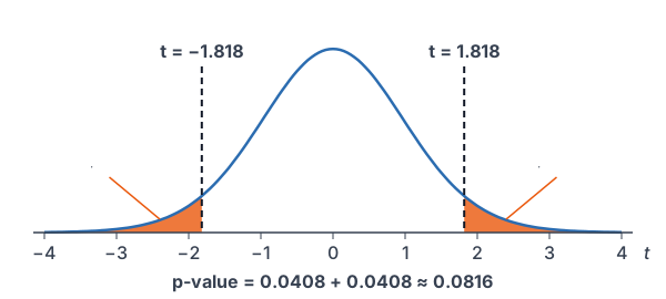
A health article says teens sleep 8 hours a night on average. A random sample of 25 students at a large school has x̄ = 7.6 hours and s = 1.1 hours, and the data show no strong skew. Is the mean for this school different from 8? Use α = 0.05.

\text{SE} = \dfrac{1.1}{\sqrt{25}} = \dfrac{1.1}{5} = 0.22

Divide s by √n.

7.6 - 8 = -0.4

Subtract μ₀ from x̄.

t = \dfrac{-0.4}{0.22} \approx -1.818

Divide by SE.

\text{df} = 25 - 1 = 24

Subtract 1 from n.

P(t \le -1.818) = \text{tcdf}(-10^{99}, -1.818, 24)

Find one tail.

\approx 0.0408

Read the calculator result.

2 \cdot 0.0408 = 0.0816

Double it for a two-sided test.

0.0816 \gt 0.05

Compare the p-value with α.

Answer: with H₀: μ = 8 and Hₐ: μ ≠ 8, the p-value is about 0.0816, so fail to reject H₀. The data don’t give convincing evidence that this school’s mean sleep time differs from 8 hours.

A t-distribution curve with 24 degrees of freedom on a t axis from −4 to 4. The areas to the left of t = −1.818 and to the right of t = 1.818 are shaded orange, each labeled 0.0408. Dashed lines mark t = −1.818 and t = 1.818. Together the two tails make the p-value, about 0.0816. — In Example 3, both tails count for a two-sided test, so the p-value is 0.0408 + 0.0408 ≈ 0.0816.

Example 4: Checking the Normal/Large Sample condition

Decide whether a one-sample t-test is safe in each case. (a) A random sample of 40 home prices is strongly right-skewed. (b) A random sample of 12 commute times has one value far above the rest.

40 \ge 30

Compare n in part (a) with 30.

12 \lt 30

Compare n in part (b) with 30.

Answer: (a) Yes. With n ≥ 30, the sampling distribution of x̄ is close to normal even though the data are skewed. (b) No. The sample is small and has an outlier, so the t procedure is not reliable. Look into the outlier or collect more data.

Example 5: Matching a test with an interval

Use the sleep data from Example 3 (x̄ = 7.6, s = 1.1, n = 25). Build a 95% confidence interval for μ. Does it agree with the test?

t^* = \text{invT}(0.975, 24) \approx 2.064

Find t* for 95% confidence with df = 24.

\text{ME} = 2.064 \cdot 0.22 \approx 0.4541

Multiply t* by SE.

7.6 - 0.4541 = 7.1459

Subtract ME.

7.6 + 0.4541 = 8.0541

Add ME.

Answer: about (7.15, 8.05) hours. The claimed value 8 is inside the interval, so it is plausible. That matches the two-sided test, which failed to reject H₀: μ = 8.

Common mistakes

Mistake	Example of the error	Fix
Using z instead of t	Finding the p-value with normalcdf when σ is unknown	Use tcdf with df = n − 1.
Wrong degrees of freedom	df = 25 for n = 25	df = n − 1 = 24.
Dividing s by n instead of √n	SE = 1.1/25 = 0.044	SE = 1.1/√25 = 0.22.
Skipping the Normal check for small samples	Using a t-test on 12 values with an outlier	Graph the data; with n < 30, there should be no strong skew or outliers.
Concluding about the sample	“The 10 cups average 15.8, so reject.”	Conclude about μ, the mean of all cups.

Related methods

Paired data

If each observation comes in a matched pair, such as before and after scores for the same student, find the differences first. Then run a one-sample t-test on the differences. That is the paired t-test, the next lesson.

Estimating the mean

A test checks one claimed value. To estimate μ with a range of plausible values, use a confidence interval for a mean. A two-sided test at α = 0.05 and a 95% interval always agree.

Practice problems

A sample has n = 16 and s = 8. Find the standard error and df.
Use Problem 1. The sample mean is 103 and H₀: μ = 100. Find t.
Use Problem 2 with Hₐ: μ > 100. Find the p-value.
A two-sided test gives t = −2.2 with df = 20. Find the p-value.
A school says its students read 30 minutes a day on average. Write H₀ and Hₐ to test whether the mean is less than that.
A company claims its bulbs last 1,200 hours on average. A random sample of 30 bulbs has x̄ = 1,176 hours and s = 60 hours. Test Hₐ: μ < 1,200 at α = 0.05.
A random sample of 10 test scores has one score far below the rest. Is a one-sample t-test appropriate?
A one-sample t-test about mean wait time gives a p-value of 0.09 with α = 0.05. Write the conclusion.
Why does this test use t instead of z?
Five randomly chosen plants grew 12, 15, 11, 14 and 13 cm. Test H₀: μ = 11 against Hₐ: μ ≠ 11 at α = 0.05. (Assume heights are roughly normal.)

Show answers

\sqrt{16} = 4

Take the square root of n.

\text{SE} = \dfrac{8}{4} = 2

Divide s by √n.

\text{df} = 16 - 1 = 15

Subtract 1 from n.

Answer: SE = 2 and df = 15

103 - 100 = 3

Subtract μ₀ from x̄.

t = \dfrac{3}{2} = 1.5

Divide by SE.

Answer: t = 1.5

P(t \ge 1.5) = \text{tcdf}(1.5, 10^{99}, 15) \approx 0.0772

Find the right-tail area.

Answer: about 0.0772

P(t \le -2.2) = \text{tcdf}(-10^{99}, -2.2, 20) \approx 0.01986

Find one tail.

2 \cdot 0.01986 \approx 0.0397

Double it for a two-sided test.

Answer: about 0.0397

Answer: H₀: μ = 30 and Hₐ: μ < 30, where μ is the true mean daily reading time of the school’s students, in minutes.

\sqrt{30} \approx 5.477

Take the square root of n.

\text{SE} = \dfrac{60}{5.477} \approx 10.95

Divide s by √n.

1176 - 1200 = -24

Subtract μ₀ from x̄.

t = \dfrac{-24}{10.95} \approx -2.192

Divide by SE.

\text{df} = 30 - 1 = 29

Subtract 1 from n.

P(t \le -2.192) = \text{tcdf}(-10^{99}, -2.192, 29) \approx 0.0183

Find the left-tail area.

0.0183 \lt 0.05

Compare with α.

Answer: p-value ≈ 0.0183, so reject H₀. There is convincing evidence that the bulbs last less than 1,200 hours on average.

10 \lt 30

Compare n with 30.

Answer: No. The sample is small and has an outlier, so the Normal/Large Sample condition fails.

0.09 \gt 0.05

Compare the p-value with α.

Answer: Fail to reject H₀. The data don’t give convincing evidence that the true mean wait time differs from the claimed value.

Answer: The population standard deviation σ is unknown, so we use s. Using s adds uncertainty, and the t-distribution’s heavier tails account for it.

10.

12 + 15 + 11 + 14 + 13 = 65

Add the values.

\bar{x} = \dfrac{65}{5} = 13

Divide by n.

1 + 4 + 4 + 1 + 0 = 10

Add the squared deviations from 13.

\dfrac{10}{4} = 2.5

Divide by n − 1.

s = \sqrt{2.5} \approx 1.581

Take the square root.

\text{SE} = \dfrac{1.581}{\sqrt{5}} \approx 0.7071

Divide s by √n.

t = \dfrac{13 - 11}{0.7071} = \dfrac{2}{0.7071}

Subtract μ₀ from x̄.

\approx 2.828

Divide by SE.

P(t \ge 2.828) = \text{tcdf}(2.828, 10^{99}, 4) \approx 0.0237

Find one tail with df = 4.

2 \cdot 0.0237 = 0.0474

Double it for a two-sided test.

0.0474 \lt 0.05

Compare with α.

Answer: p-value ≈ 0.0474, so reject H₀. There is convincing evidence that the mean height differs from 11 cm (just barely at α = 0.05).

One-sample t-test FAQ

What is the formula for a one-sample t-test?

The test statistic is t = (x̄ − μ₀) ÷ (s/√n), with df = n − 1. The p-value is the matching tail area under the t-distribution with those degrees of freedom.

When do you use a t-test instead of a z-test?

Use a t-test for a mean when the population standard deviation σ is unknown, which is almost always. A z-test for a mean needs σ, which you rarely know.

What are the conditions for a one-sample t-test?

The data must come from a random sample or experiment, the sample must be at most 10% of the population, and the population must be roughly normal or n must be at least 30.

How do you do a one-sample t-test on a TI-84?

Press STAT, choose TESTS, then 2:T-Test. Pick Data or Stats, enter μ₀ and your sample information, choose the direction of Hₐ, then choose Calculate.

Summary

Use a one-sample t-test to check a claim H₀: μ = μ₀ when σ is unknown.
t = (x̄ − μ₀) ÷ (s/√n), with df = n − 1.
Check Random, 10% and Normal/Large Sample (n ≥ 30, or no strong skew or outliers).
Find the p-value with tcdf in the tail that matches Hₐ, and compare it with α.
State the conclusion in context about the population mean μ.

Previous lesson: Two-Proportion z-Test

Next lesson: Paired t-Test

Back to the Statistics Index