
Confidence Interval for a Mean
A confidence interval for a mean gives a range of plausible values for a population mean μ. When σ is unknown, you build a one-sample t-interval: x̄ ± t* · s/√n, with df = n − 1. The sample mean x̄ is the center, and the margin of error t* · s/√n sets the width.
Before this lesson: Confidence Intervals, Sampling Distribution of a Sample Mean and t-Distribution
What a t-interval does
A sample mean x̄ is your best single guess for μ. But a different sample would give a different x̄. The interval adds a cushion on each side to cover that sample-to-sample change.
The cushion is the margin of error. It is a critical value times the standard error s/√n, which measures how much x̄ typically varies. Because you use s in place of the unknown σ, the critical value comes from the t-distribution, not the normal curve.
The result is called a one-sample t-interval. It works the same way as the confidence interval for a proportion: estimate ± margin of error.
Confidence interval for a mean formula
\bar{x} \pm t^* \cdot \dfrac{s}{\sqrt{n}} \qquad df = n - 1- x̄ is the sample mean and s is the sample standard deviation.
- n is the sample size, and s/√n is the standard error (SE).
- t* is the t critical value for your confidence level with df = n − 1. For 95%, t* = invT(0.975, df).
- The margin of error is ME = t* · SE.
Conditions
- Random: the data come from a random sample or a randomized experiment.
- 10%: when sampling without replacement, n is at most 10% of the population.
- Normal/Large Sample: the population is roughly normal, or n ≥ 30. For a small sample, graph the data and check for no strong skew and no outliers.
The n ≥ 30 rule comes from the central limit theorem. For a small sample, the t-interval is only safe when the data look roughly symmetric (see the IQR rule for outliers).
Four steps
- State: name the parameter μ and the confidence level.
- Plan: name the method (one-sample t-interval) and check the three conditions.
- Do: find df, t*, SE and ME, then compute x̄ − ME and x̄ + ME.
- Conclude: interpret the interval in context.
Calculator: on a TI-84, press STAT, choose TESTS, then 8:TInterval. Choose Stats to enter x̄, s and n, or Data to use a list. The calculator finds t* for you.
Confidence interval for a mean examples
Example 1: Build a 95% t-interval
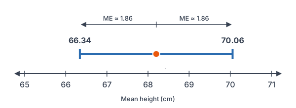
A random sample of 25 sunflower plants from a large field has mean height x̄ = 68.2 cm and standard deviation s = 4.5 cm. A dot plot of the heights shows no strong skew and no outliers. Build a 95% confidence interval for the mean height μ.
Conditions: the sample is random, 25 plants is far less than 10% of the field, and the data show no strong skew or outliers.
df = 25 - 1 = 24
Subtract 1 from n.
t^* = \text{invT}(0.975, 24) \approx 2.064Use left area 0.975 with df = 24.
\sqrt{25} = 5Find √n (see square roots).
\text{SE} = \dfrac{4.5}{5} = 0.9Divide s by √n.
\text{ME} = 2.064 \cdot 0.9 = 1.8576Multiply t* by SE.
68.2 - 1.8576 = 66.3424
Subtract ME from x̄.
68.2 + 1.8576 = 70.0576
Add ME to x̄.
Answer: about (66.34, 70.06) cm. We are 95% confident that the mean height of all sunflowers in the field is between 66.34 cm and 70.06 cm.
Example 2: Start from raw data
Ten randomly chosen students at a large high school report how many hours they slept last night: 6.5, 7.0, 5.5, 8.0, 6.0, 7.5, 6.5, 7.0, 5.0, 6.0. The values are roughly symmetric with no outliers. Build a 90% confidence interval for the mean sleep time.
6.5 + 7.0 + 5.5 + 8.0 + 6.0 + 7.5 + 6.5 + 7.0 + 5.0 + 6.0 = 65
Add the 10 values.
\bar{x} = \dfrac{65}{10} = 6.5Divide by n to get the mean.
| Value | Deviation (x − 6.5) | Squared deviation |
|---|---|---|
| 6.5 | 0 | 0 |
| 7.0 | 0.5 | 0.25 |
| 5.5 | −1 | 1 |
| 8.0 | 1.5 | 2.25 |
| 6.0 | −0.5 | 0.25 |
| 7.5 | 1 | 1 |
| 6.5 | 0 | 0 |
| 7.0 | 0.5 | 0.25 |
| 5.0 | −1.5 | 2.25 |
| 6.0 | −0.5 | 0.25 |
0 + 0.25 + 1 + 2.25 + 0.25 + 1 + 0 + 0.25 + 2.25 + 0.25 = 7.5
Add the squared deviations from the table.
s^2 = \dfrac{7.5}{9} \approx 0.8333Divide by n − 1 (see sample standard deviation).
s = \sqrt{0.8333} \approx 0.9129Take the square root.
df = 10 - 1 = 9
Subtract 1 from n.
t^* = \text{invT}(0.95, 9) \approx 1.833For 90%, use left area 0.95.
\sqrt{10} \approx 3.162Find √n.
\text{SE} = \dfrac{0.9129}{3.162} \approx 0.2887Divide s by √n.
\text{ME} = 1.833 \cdot 0.2887 \approx 0.5292Multiply t* by SE.
6.5 - 0.5292 = 5.9708
Subtract ME from x̄.
6.5 + 0.5292 = 7.0292
Add ME to x̄.
Answer: about (5.97, 7.03) hours. We are 90% confident that the mean sleep time for all students at the school is between 5.97 and 7.03 hours. TInterval with Data gives the same result.
Example 3: Raise the confidence level
Use the sunflower data from Example 1 (x̄ = 68.2, s = 4.5, n = 25). Build a 99% interval and compare its width with the 95% interval.
t^* = \text{invT}(0.995, 24) \approx 2.797For 99%, use left area 0.995.
\text{ME} = 2.797 \cdot 0.9 = 2.5173Multiply t* by SE = 0.9 from Example 1.
68.2 - 2.5173 = 65.6827
Subtract ME from x̄.
68.2 + 2.5173 = 70.7173
Add ME to x̄.
2 \cdot 2.5173 = 5.0346
Width of the 99% interval.
2 \cdot 1.8576 = 3.7152
Width of the 95% interval.
Answer: about (65.68, 70.72) cm, with width 5.03 cm instead of 3.72 cm. More confidence costs a wider interval.
Example 4: Checking a battery claim (word problem)
A phone maker says its battery lasts 10 hours on average. A consumer group tests a random sample of 20 phones and finds x̄ = 9.4 hours and s = 1.1 hours. A dot plot of the 20 times is roughly symmetric with no outliers. Build a 95% interval. Is the claim plausible?
df = 20 - 1 = 19
Subtract 1 from n.
t^* = \text{invT}(0.975, 19) \approx 2.093Use left area 0.975 with df = 19.
\sqrt{20} \approx 4.472Find √n.
\text{SE} = \dfrac{1.1}{4.472} \approx 0.2460Divide s by √n.
\text{ME} = 2.093 \cdot 0.2460 \approx 0.5149Multiply t* by SE.
9.4 - 0.5149 = 8.8851
Subtract ME from x̄.
9.4 + 0.5149 = 9.9149
Add ME to x̄.
Answer: about (8.89, 9.91) hours. The claimed mean of 10 hours is outside the interval, so it is not a plausible value. The data give good evidence that the true mean battery life is less than 10 hours.
Example 5: Work backward from an interval
A report gives a 95% confidence interval of (42.1, 47.9) for a mean, from a sample of 16. Find x̄, the margin of error and the sample standard deviation s.
\bar{x} = \dfrac{42.1 + 47.9}{2} = \dfrac{90}{2}Add the endpoints.
= 45
Divide by 2; x̄ is the midpoint.
\text{ME} = 47.9 - 45 = 2.9Subtract x̄ from the upper endpoint.
t^* = \text{invT}(0.975, 15) \approx 2.131Use df = 16 − 1 = 15.
\text{SE} = \dfrac{2.9}{2.131} \approx 1.361Divide ME by t*.
s = 1.361 \cdot 4 = 5.444
Multiply SE by √16 = 4.
Answer: x̄ = 45, ME = 2.9 and s ≈ 5.44. Since SE = s/√n, you undo it by multiplying by √n.
Common mistakes
| Mistake | Example of the error | Fix |
|---|---|---|
| Using z* instead of t* | 1.96 for a mean when only s is known | Use t* from invT with df = n − 1. |
| Using df = n | invT(0.975, 25) for n = 25 | df = n − 1 = 24. |
| Dividing s by n instead of √n | SE = 4.5/25 = 0.18 | SE = 4.5/√25 = 0.9. |
| Skipping the Normal condition | t-interval for 12 values with a big outlier | For n under 30, graph the data first. |
| Saying 95% of the data fall in the interval | “95% of plants are 66.34 to 70.06 cm” | The interval estimates the mean μ, not single values. |
Related methods
When σ is known: the z-interval
If you somehow know the population standard deviation σ, use \bar{x} \pm z^* \cdot \sigma/\sqrt{n} with z* from the normal curve. This is rare in real studies, so the t-interval is the standard method.
Paired data
For matched pairs, such as before-and-after scores for the same people, find each pair’s difference first. Then build a one-sample t-interval on those differences (see matched pairs design).
Planning the sample size
To reach a chosen margin of error, solve ME = z*σ/√n for n, using a guess for σ. The margin of error lesson shows the steps.
Practice problems
- A sample has n = 36. Find df and t* for a 95% confidence interval.
- A random sample of 16 has x̄ = 50 and s = 8. Build a 95% confidence interval for μ.
- A random sample of 25 has x̄ = 12.4 and s = 3. Build a 99% confidence interval for μ.
- A 95% confidence interval for a mean is (18.6, 23.4). Find x̄ and the margin of error.
- A random sample of 8 has x̄ = 30 and s = 4, and the data look roughly normal. Build a 95% confidence interval.
- A random sample of 12 home prices is strongly skewed right with one very high outlier. Is a t-interval safe? Explain.
- A 95% confidence interval for the mean daily screen time of teens at a school is (3.1, 3.9) hours. Interpret it.
- A 95% confidence interval for mean commute time is (24.2, 28.6) minutes. Is 30 minutes a plausible mean? Is 25 minutes?
- A random sample of 30 has x̄ = 72 and s = 6. Build a 90% confidence interval for μ.
- Use Example 1 (s = 4.5). If n grows from 25 to 100, find the new 95% margin of error. About how does it compare with 1.8576?
Show answers
1.
df = 36 - 1 = 35
Subtract 1 from n.
t^* = \text{invT}(0.975, 35) \approx 2.030Left area 0.975 with df = 35.
Answer: df = 35 and t* ≈ 2.030
2.
t^* = \text{invT}(0.975, 15) \approx 2.131df = 16 − 1 = 15.
\text{SE} = \dfrac{8}{\sqrt{16}} = \dfrac{8}{4}Divide s by √n, using √16 = 4.
= 2
Divide.
\text{ME} = 2.131 \cdot 2 = 4.262Multiply t* by SE.
50 - 4.262 = 45.738
Subtract ME from x̄.
50 + 4.262 = 54.262
Add ME to x̄.
Answer: about (45.74, 54.26)
3.
t^* = \text{invT}(0.995, 24) \approx 2.797df = 24; left area 0.995 for 99%.
\text{SE} = \dfrac{3}{\sqrt{25}} = \dfrac{3}{5}Divide s by √n, using √25 = 5.
= 0.6
Divide.
\text{ME} = 2.797 \cdot 0.6 = 1.6782Multiply t* by SE.
12.4 - 1.6782 = 10.7218
Subtract ME from x̄.
12.4 + 1.6782 = 14.0782
Add ME to x̄.
Answer: about (10.72, 14.08)
4.
\bar{x} = \dfrac{18.6 + 23.4}{2} = \dfrac{42}{2}Add the endpoints.
= 21
Divide by 2.
\text{ME} = 23.4 - 21 = 2.4Subtract x̄ from the upper endpoint.
Answer: x̄ = 21 and ME = 2.4
5.
t^* = \text{invT}(0.975, 7) \approx 2.365df = 8 − 1 = 7.
\sqrt{8} \approx 2.828Find √n.
\text{SE} = \dfrac{4}{2.828} \approx 1.414Divide s by √n.
\text{ME} = 2.365 \cdot 1.414 \approx 3.344Multiply t* by SE.
30 - 3.344 = 26.656
Subtract ME from x̄.
30 + 3.344 = 33.344
Add ME to x̄.
Answer: about (26.66, 33.34)
6.
The sample is small (12 is under 30), and the data are strongly skewed with an outlier, so the Normal/Large Sample condition fails.
Answer: No. A t-interval is not safe for these data.
7.
The interval estimates the mean for all teens at the school, not single students.
Answer: We are 95% confident that the mean daily screen time of all teens at the school is between 3.1 and 3.9 hours.
8.
30 is greater than 28.6, so it is outside the interval. 25 is between 24.2 and 28.6.
Answer: 30 minutes is not plausible; 25 minutes is plausible.
9.
t^* = \text{invT}(0.95, 29) \approx 1.699df = 29; left area 0.95 for 90%.
\sqrt{30} \approx 5.477Find √n.
\text{SE} = \dfrac{6}{5.477} \approx 1.0955Divide s by √n.
\text{ME} = 1.699 \cdot 1.0955 \approx 1.8613Multiply t* by SE.
72 - 1.8613 = 70.1387
Subtract ME from x̄.
72 + 1.8613 = 73.8613
Add ME to x̄.
Answer: about (70.14, 73.86)
10.
t^* = \text{invT}(0.975, 99) \approx 1.984df = 100 − 1 = 99.
\text{SE} = \dfrac{4.5}{\sqrt{100}} = \dfrac{4.5}{10}Divide s by √n, using √100 = 10.
= 0.45
Divide.
\text{ME} = 1.984 \cdot 0.45 = 0.8928Multiply t* by SE.
\dfrac{0.8928}{1.8576} \approx 0.481Compare with the old ME.
Answer: ME ≈ 0.893, a little less than half of 1.8576. Four times the sample size halves the SE, and t* also shrinks a bit.
Confidence interval for a mean FAQ
What is the formula for a confidence interval for a mean?
When σ is unknown, use x̄ ± t* · s/√n, where t* comes from the t-distribution with df = n − 1. The part after ± is the margin of error.
When do you use t instead of z for a confidence interval?
Use t for a mean whenever you estimate σ with the sample standard deviation s, which is almost always. Use z only if σ is truly known, and always use z for proportions.
What does a 95% confidence interval for a mean tell you?
It gives a range of plausible values for the population mean. The 95% means the method captures the true mean in about 95% of all possible samples.
What sample size do you need for a t-interval?
Any size works if the population is roughly normal. If you don’t know the shape, n ≥ 30 is the usual rule; for smaller samples, check a graph of the data for strong skew and outliers.
Summary
- A confidence interval for a mean is x̄ ± t* · s/√n, with df = n − 1.
- Check Random, 10% and Normal/Large Sample before you build it.
- Find t* with invT(left area, df) or a t-table; for 95%, the left area is 0.975.
- Higher confidence or a smaller sample gives a wider interval.
- Interpret it as a range of plausible values for the population mean μ, not for single values.
Previous lesson: t-Distribution
Next lesson: Confidence Interval for a Difference in Proportions
Back to the Statistics Index