
Sampling Distribution of a Sample Mean
The sampling distribution of a sample mean describes how the sample mean x̄ varies from one random sample to the next. Its mean is the population mean μ, and its standard deviation is σ/√n. It is normal when the population is normal, and approximately normal when n is at least 30.
Before this lesson: Central Limit Theorem, Sampling Distribution of a Sample Proportion and Normal Probability Calculations
What the sampling distribution of x̄ shows
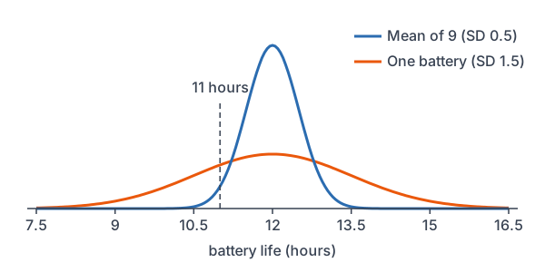
A phone battery lasts 12 hours on average, with a standard deviation of 1.5 hours. One battery might last 10.4 hours. But if you test 9 batteries and average them, the short and long ones balance out. The average will usually land much closer to 12.
The sampling distribution of x̄ is the distribution of the sample means from all possible samples of the same size. It has the same center as the population but a smaller spread. That is why one unusual value is common, while an unusual average is rare.
Sampling distribution of a sample mean formula
\mu_{\bar{x}} = \mu \qquad \sigma_{\bar{x}} = \dfrac{\sigma}{\sqrt{n}}Before you use these facts, check three conditions:
- Random: the data come from a random sample or a randomized experiment.
- 10% condition: the sample is less than 10% of the population, so the σ/√n formula is accurate.
- Normal/Large Sample: the population is normal, or n ≥ 30. Then x̄ is normal or approximately normal by the central limit theorem.
The standard deviation σ/√n is also called the standard error of the mean in many textbooks. Because n is under a square root, you need 4 times the sample size to cut it in half.
Calculator: on a TI-84, use normalcdf(lower, upper, μ, σ/√n) for a probability and invNorm(area, μ, σ/√n) for a cutoff. In Desmos, use normaldist(μ, σ/√n).
Sampling distribution of a sample mean examples
Example 1: Describe the sampling distribution
Battery life is normal with mean 12 hours and standard deviation 1.5 hours. A random sample of 9 batteries is tested. Describe the sampling distribution of x̄.
\mu_{\bar{x}} = \mu = 12The mean of x̄ equals the population mean.
\sqrt{9} = 3Find the square root of n (see square roots).
\sigma_{\bar{x}} = \dfrac{1.5}{3} = 0.5Divide σ by √n.
Answer: x̄ is normal, because the population is normal, with mean 12 hours and standard deviation 0.5 hours.
Example 2: One value vs. a sample mean
Use Example 1. Find the probability that (a) one battery lasts less than 11 hours, and (b) the mean of 9 batteries is less than 11 hours.
z = \dfrac{11 - 12}{1.5} = \dfrac{-1}{1.5}(a) Use σ for one battery: subtract.
\approx -0.67
Divide.
P(Z \lt -0.67) = 0.2514
Read the z-table (see standard normal distribution).
z = \dfrac{11 - 12}{0.5} = \dfrac{-1}{0.5}(b) Use σ/√n for the mean: subtract.
= -2
Divide.
P(Z \lt -2) = 0.0228
Read the z-table.
Answer: (a) about 0.2514; (b) about 0.0228. One short battery happens about 1 time in 4, but a short average of 9 happens only about 2 times in 100.
Example 3: Check the conditions, then find a probability
A shipment has 2,000 cereal boxes. Box weights have mean 510 grams and standard deviation 8 grams, but their shape is unknown. An inspector weighs a random sample of 40 boxes. What is the probability that the sample mean is less than 508 grams?
0.10(2000) = 200
10% condition: find 10% of the shipment.
40 \lt 200
The sample is less than 10% of the shipment.
40 \ge 30
The sample is large, so x̄ is approximately normal.
\sqrt{40} \approx 6.325Find √n.
\sigma_{\bar{x}} = \dfrac{8}{6.325} \approx 1.265Divide σ by √n.
z = \dfrac{508 - 510}{1.265} = \dfrac{-2}{1.265}Change 508 to a z-score: subtract.
\approx -1.58
Divide.
P(Z \lt -1.58) = 0.0571
Read the z-table.
Answer: about 0.0571. All three conditions hold, since the sample is random, small compared with the shipment, and large.
Example 4: Find a cutoff for x̄
Use Example 1. Find the sample mean that only 5% of samples of 9 batteries will beat.
z = 1.645
The top 5% starts at the 95th percentile, where z = 1.645 (see z-scores).
\bar{x} = \mu + z \sigma_{\bar{x}}Solve the z-score formula for x̄.
= 12 + 1.645(0.5)
Substitute.
= 12 + 0.8225
Multiply.
= 12.8225
Add.
Answer: about 12.82 hours. Only 5% of samples of 9 batteries average more than 12.82 hours.
Example 5: Commute times (word problem)
In a large city, commute times have mean 28 minutes and standard deviation 10 minutes, and they are skewed right. A random sample of 64 commuters is taken. What is the probability that their mean commute is between 26 and 30 minutes?
64 \ge 30
The sample is large, so x̄ is approximately normal even though commutes are skewed.
\sigma_{\bar{x}} = \dfrac{10}{\sqrt{64}} = \dfrac{10}{8}Divide σ by √n, using √64 = 8.
= 1.25
Divide.
z = \dfrac{26 - 28}{1.25} = \dfrac{-2}{1.25}Lower z: subtract.
= -1.6
Divide.
z = \dfrac{30 - 28}{1.25} = \dfrac{2}{1.25}Upper z: subtract.
= 1.6
Divide.
0.9452 - 0.0548 = 0.8904
Subtract the left areas: P(Z \lt 1.6) = 0.9452 and P(Z \lt -1.6) = 0.0548.
Answer: about 0.8904. The city has far more than 640 commuters, so the 10% condition holds.
Common mistakes
| Mistake | Example of the error | Fix |
|---|---|---|
| Using σ for a sample mean | z = (11 − 12)/1.5 for the mean of 9 batteries | For x̄, divide by σ/√n = 0.5. |
| Using σ/√n for one value | z = (11 − 12)/0.5 for one battery | One value comes from the population, so use σ. |
| Dividing by n instead of √n | σ of x̄ = 1.5/9 | Divide by √9 = 3. |
| Using a normal model for a small sample from a skewed population | A normal model for x̄ with n = 12 from skewed data | Use n ≥ 30, or a normal population. |
| Skipping the 10% condition | Sampling 50 of 400 items and using σ/√n | 50 is more than 10% of 400, so the formula overstates the spread. |
Related methods
Means vs. proportions
The sampling distribution of a sample proportion follows the same pattern. Its center is p, its spread is \sqrt{p(1 - p)/n}, and its shape is checked with Large Counts instead of n ≥ 30.
When σ is unknown
In real studies, σ is usually unknown, so it is replaced with the sample standard deviation s (see standard deviation). Then the z-score is replaced with a t-score, which a later lesson on the t-distribution explains.
Practice problems
- A normal population has μ = 80 and σ = 12. For n = 16, describe the sampling distribution of x̄.
- Use Problem 1. Find P(\bar{x} \gt 85).
- Use Problem 1. Find the probability that one value is greater than 85.
- A population is strongly skewed, and n = 12. Can you use a normal model for x̄?
- With σ = 20, what sample size makes the standard deviation of x̄ equal to 4?
- The sample size grows from 25 to 100. What happens to the standard deviation of x̄?
- A sample of 50 items is taken from a batch of 400. Is the 10% condition met?
- A population has μ = 200 and σ = 30, with unknown shape. For n = 36, find P(190 \lt \bar{x} \lt 210).
- Use Problem 8. Find the sample mean that marks the bottom 10% of samples.
- Light bulbs from a large batch last a mean of 1,200 hours with standard deviation 150 hours. For a random sample of 50 bulbs, find the probability that the mean life is less than 1,170 hours.
Show answers
1.
\mu_{\bar{x}} = 80Same as the population mean.
\sqrt{16} = 4Find √n.
\sigma_{\bar{x}} = \dfrac{12}{4} = 3Divide σ by √n.
Answer: normal, with mean 80 and standard deviation 3
2.
z = \dfrac{85 - 80}{3} = \dfrac{5}{3}Change 85 to a z-score: subtract.
\approx 1.67
Divide.
1 - 0.9525 = 0.0475
P(Z \lt 1.67) = 0.9525, so take the right area.
Answer: about 0.0475
3.
z = \dfrac{85 - 80}{12} = \dfrac{5}{12}One value uses σ: subtract.
\approx 0.42
Divide.
1 - 0.6628 = 0.3372
P(Z \lt 0.42) = 0.6628, so take the right area.
Answer: about 0.3372
4.
The sample is small, and the population is strongly skewed.
Answer: no
5.
\dfrac{20}{\sqrt{n}} = 4Set the standard deviation of x̄ equal to 4.
20 = 4\sqrt{n}Multiply both sides by √n.
\sqrt{n} = 5Divide both sides by 4.
n = 25
Square both sides.
Answer: n = 25
6.
\sqrt{25} = 5 \text{ and } \sqrt{100} = 10Find √n for each sample size.
\dfrac{\sigma}{10} = \dfrac{1}{2} \cdot \dfrac{\sigma}{5}Compare σ/10 with σ/5.
Answer: it is cut in half
7.
0.10(400) = 40
Find 10% of the batch.
50 \gt 40
Compare the sample size.
Answer: no, the sample is more than 10% of the batch
8.
36 \ge 30
The sample is large, so x̄ is approximately normal.
\sigma_{\bar{x}} = \dfrac{30}{\sqrt{36}} = \dfrac{30}{6}Divide σ by √n, using √36 = 6.
= 5
Divide.
z = \dfrac{190 - 200}{5} = \dfrac{-10}{5}Lower z: subtract.
= -2
Divide.
z = \dfrac{210 - 200}{5} = \dfrac{10}{5}Upper z: subtract.
= 2
Divide.
0.9772 - 0.0228 = 0.9544
Subtract the left areas: P(Z \lt 2) = 0.9772 and P(Z \lt -2) = 0.0228.
Answer: about 0.9544
9.
z = -1.28
The 10th percentile of the standard normal curve.
\bar{x} = 200 + (-1.28)(5)Substitute into x̄ = μ + zσ of x̄.
= 200 - 6.4
Multiply.
= 193.6
Subtract.
Answer: about 193.6
10.
\sqrt{50} \approx 7.071Find √n.
\sigma_{\bar{x}} = \dfrac{150}{7.071} \approx 21.21Divide σ by √n.
z = \dfrac{1170 - 1200}{21.21} = \dfrac{-30}{21.21}Change 1,170 to a z-score: subtract.
\approx -1.41
Divide.
P(Z \lt -1.41) = 0.0793
Read the z-table.
Answer: about 0.0793
Sampling distribution of a sample mean FAQ
What is the mean of the sampling distribution of the sample mean?
It equals the population mean μ. So x̄ is an unbiased estimator of μ.
What is the standard error of the mean?
It is the standard deviation of the sampling distribution of x̄, σ/√n. When σ is unknown, it is estimated with s/√n.
When is the sampling distribution of x̄ normal?
It is exactly normal when the population is normal. It is approximately normal when n ≥ 30, by the central limit theorem, even if the population is skewed.
Why is the sampling distribution of x̄ narrower than the population?
Averages balance out high and low values, so they vary less than single values. The spread shrinks by a factor of √n.
Summary
- The mean of x̄ is μ, and its standard deviation is σ/√n.
- Check Random, 10% and Normal/Large Sample before using a normal model.
- Use σ for one value and σ/√n for a sample mean.
- Find cutoffs with x̄ = μ + zσ/√n.
- Quadrupling n cuts the standard deviation of x̄ in half.
Previous lesson: Sampling Distribution of a Sample Proportion
Next lesson: Sampling Distributions for Differences
Back to the Statistics Index