Sampling Distribution of a Sample Proportion

The sampling distribution of a sample proportion describes how the sample proportion p̂ varies from one random sample to the next. Its mean is the population proportion p, and its standard deviation is $\sqrt{p(1 - p)/n}$ . When np and n(1 − p) are both at least 10, its shape is approximately normal.

Before this lesson: Sampling Distributions, Central Limit Theorem and Binomial Distribution

What the sampling distribution of p̂ shows

Suppose 40% of the students at a large college commute, so p = 0.40. If you survey 150 random students, you might get p̂ = 0.37. Another sample might give 0.43. The sample proportion p̂ is the number of successes divided by n.

Picture taking every possible sample of 150 and finding p̂ for each one. The distribution of all those p̂ values is the sampling distribution of p̂. It tells you which sample results are typical and which would be surprising.

Three facts describe it: where it is centered, how spread out it is, and its shape. Each fact comes with a condition you should check.

A normal curve for the sample proportion with p = 0.40 and n = 150. The horizontal axis is marked from 0.28 to 0.52 in steps of 0.04, which is one standard deviation. The curve peaks at 0.40. The region to the right of 0.46 is shaded and labeled 0.0668. — For p = 0.40 and n = 150, p̂ is centered at 0.40 with standard deviation 0.04. A sample with p̂ above 0.46 happens about 6.7% of the time.

Sampling distribution of a sample proportion formula

\mu_{\hat{p}} = p \qquad \sigma_{\hat{p}} = \sqrt{\dfrac{p(1 - p)}{n}}

Center: the mean of p̂ equals p. So p̂ is an unbiased estimator of p.
Spread: the standard deviation of p̂ is $\sqrt{p(1 - p)/n}$ . Use this only when the sample is less than 10% of the population (the 10% condition), so the observations are close to independent.
Shape: p̂ is approximately normal when np ≥ 10 and n(1 − p) ≥ 10 (the Large Counts condition). These are the expected numbers of successes and failures.

Larger samples make p̂ less variable. Because n is under a square root, you need 4 times the sample size to cut the standard deviation in half.

Calculator: for a probability about p̂ on a TI-84, use normalcdf(lower, upper, p, σ), where σ is the standard deviation of p̂. In Desmos, use normaldist(p, σ).cdf(a, b).

Sampling distribution of a sample proportion examples

Example 1: Find the mean and standard deviation of p̂

At a large college, 40% of students commute. A random sample of 150 students is taken. Find the mean and standard deviation of p̂.

\mu_{\hat{p}} = p = 0.40

The mean of p̂ equals the population proportion.

1 - 0.40 = 0.60

Find 1 − p.

0.40(0.60) = 0.24

Multiply p by 1 − p.

\dfrac{0.24}{150} = 0.0016

Divide by n.

\sigma_{\hat{p}} = \sqrt{0.0016} = 0.04

Take the square root (see square roots).

Answer: the mean of p̂ is 0.40 and its standard deviation is 0.04. Sample proportions typically land about 0.04 away from 0.40.

Example 2: Check the conditions

Use Example 1. The college has 12,000 students. (a) Check the 10% condition. (b) Check the Large Counts condition. (c) A different survey studies a trait with p = 0.03 and n = 200. Is p̂ approximately normal?

0.10(12{,}000) = 1200

(a) Find 10% of the population.

150 \lt 1200

The sample is less than 10% of the population, so the condition is met.

np = 150(0.40) = 60

(b) Expected number of successes.

n(1 - p) = 150(0.60) = 90

Expected number of failures.

60 \ge 10 \text{ and } 90 \ge 10

Both counts are at least 10, so p̂ is approximately normal.

np = 200(0.03) = 6

6 \lt 10

The Large Counts condition fails.

Answer: (a) met; (b) met, so the normal model is fine; (c) no. With only about 6 expected successes, the distribution of p̂ is skewed right.

Example 3: Probability for a sample proportion

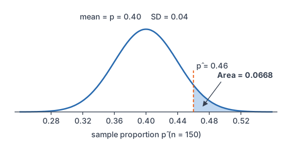
Use Example 1. What is the probability that more than 46% of the 150 students in the sample commute?

z = \dfrac{0.46 - 0.40}{0.04}

Change 0.46 to a z-score, using the standard deviation of p̂.

= \dfrac{0.06}{0.04}

Subtract.

= 1.5

Divide.

P(Z \lt 1.5) = 0.9332

Read the z-table (see standard normal distribution).

1 - 0.9332 = 0.0668

More than 0.46 is the right area (see complement rule).

Answer: about 0.0668. A sample result above 46% would happen in about 1 of every 15 samples.

Example 4: Probability between two values

A national survey reports that 72% of adults use a streaming service. In a random sample of 400 adults, what is the probability that p̂ is between 0.70 and 0.75?

400(0.72) = 288 \text{ and } 400(0.28) = 112

Both counts are at least 10, so p̂ is approximately normal.

0.72(0.28) = 0.2016

Multiply p by 1 − p.

\dfrac{0.2016}{400} = 0.000504

Divide by n.

\sigma_{\hat{p}} = \sqrt{0.000504} \approx 0.02245

Take the square root.

z = \dfrac{0.70 - 0.72}{0.02245} = \dfrac{-0.02}{0.02245}

Lower z: subtract.

\approx -0.89

Divide.

z = \dfrac{0.75 - 0.72}{0.02245} = \dfrac{0.03}{0.02245}

Upper z: subtract.

\approx 1.34

Divide.

0.9099 - 0.1867 = 0.7232

Subtract the left areas: $P(Z \lt 1.34) = 0.9099$ and $P(Z \lt -0.89) = 0.1867$ .

Answer: about 0.72. The population of U.S. adults is far more than 10 times 400, so the 10% condition is met.

Example 5: Is a claim believable? (word problem)

A delivery company claims that 90% of its packages arrive on time. A customer group tracks a random sample of 250 packages, and only 212 arrive on time. If the claim is true, how unusual is a result this low?

\hat{p} = \dfrac{212}{250} = 0.848

Find the sample proportion.

250(0.90) = 225 \text{ and } 250(0.10) = 25

Both counts are at least 10, so use a normal model.

0.90(0.10) = 0.09

Multiply p by 1 − p.

\dfrac{0.09}{250} = 0.00036

Divide by n.

\sigma_{\hat{p}} = \sqrt{0.00036} \approx 0.01897

Take the square root.

z = \dfrac{0.848 - 0.90}{0.01897} = \dfrac{-0.052}{0.01897}

Change 0.848 to a z-score: subtract.

\approx -2.74

Divide.

P(Z \lt -2.74) = 0.0031

Read the z-table.

Answer: about 0.0031. If 90% really arrived on time, a sample this low would happen only about 3 times in 1,000 samples. That is strong evidence the true on-time rate is below 90%. Hypothesis tests later in the course make this reasoning formal.

Common mistakes

Mistake	Example of the error	Fix
Using p̂ in place of p in the formula	With p = 0.90 and p̂ = 0.848, using 0.848(0.152) for the spread	When p is known or claimed, use p to find the mean and standard deviation of p̂.
Forgetting the square root	σ of p̂ = 0.24/150 = 0.0016	Take the square root: $\sqrt{0.0016} = 0.04$ .
Checking Large Counts with p̂ alone	“p̂ = 0.4, which is at least 10”	Check the counts np and n(1 − p), not the proportion.
Skipping the 10% condition	Sampling 80 of 500 seniors and using the formula	80 is more than 10% of 500, so the formula overstates the spread.
Thinking a bigger population needs a bigger sample	“A national poll needs a much larger n than a city poll”	The spread depends on n, not on the population size, as long as the 10% condition holds.

Related methods

Connection to the binomial distribution

The number of successes X in the sample is a binomial count, and p̂ = X/n. Dividing the binomial mean np and standard deviation $\sqrt{np(1 - p)}$ by n gives the formulas above. The Large Counts check is the same one used for the normal approximation to the binomial.

What comes next

Confidence intervals and tests for a proportion start from this sampling distribution. When p is unknown, they replace p with p̂ in the standard deviation formula. The next lesson, Sampling Distribution of a Sample Mean, does the same work for means, and normal probability calculations cover the z-score steps in more detail.

Practice problems

A population proportion is p = 0.25, and n = 300. Find the mean and standard deviation of p̂.
Use Problem 1. Check the Large Counts condition.
A trait has p = 0.05, and n = 120. Is p̂ approximately normal?
Use Problem 1. Find $P(\hat{p} \lt 0.20)$ .
Use Problem 1. Find $P(\hat{p} \gt 0.30)$ .
Use Problem 1. Find $P(0.22 \lt \hat{p} \lt 0.28)$ .
If p = 0.5, how large must n be for the standard deviation of p̂ to equal 0.02?
A teacher samples 80 of the 500 seniors at a school. Is the 10% condition met?
In a large town, 64% of voters support a new park. In a random poll of 225 voters, find the probability that less than 60% support it.
Use Problem 9. The poll grows to 900 voters. Find the new standard deviation of p̂.

Show answers

\mu_{\hat{p}} = 0.25

The mean of p̂ equals p.

0.25(0.75) = 0.1875

Multiply p by 1 − p.

\dfrac{0.1875}{300} = 0.000625

Divide by n.

\sigma_{\hat{p}} = \sqrt{0.000625} = 0.025

Take the square root.

Answer: mean 0.25, standard deviation 0.025

np = 300(0.25) = 75

Expected successes.

n(1 - p) = 300(0.75) = 225

Expected failures.

Answer: both counts are at least 10, so the condition is met

np = 120(0.05) = 6

Expected successes.

6 \lt 10

The Large Counts condition fails.

Answer: no, p̂ is skewed right

z = \dfrac{0.20 - 0.25}{0.025} = \dfrac{-0.05}{0.025}

Change 0.20 to a z-score: subtract.

= -2

Divide.

P(Z \lt -2) = 0.0228

Read the z-table.

Answer: about 0.0228

z = \dfrac{0.30 - 0.25}{0.025} = \dfrac{0.05}{0.025}

Change 0.30 to a z-score: subtract.

= 2

Divide.

1 - 0.9772 = 0.0228

$P(Z \lt 2) = 0.9772$ , so take the right area.

Answer: about 0.0228

z = \dfrac{0.22 - 0.25}{0.025} = \dfrac{-0.03}{0.025}

Lower z: subtract.

= -1.2

Divide.

z = \dfrac{0.28 - 0.25}{0.025} = \dfrac{0.03}{0.025}

Upper z: subtract.

= 1.2

Divide.

0.8849 - 0.1151 = 0.7698

Subtract the left areas.

Answer: about 0.7698

\sqrt{\dfrac{0.5(0.5)}{n}} = 0.02

Set the standard deviation of p̂ equal to 0.02.

\dfrac{0.5(0.5)}{n} = 0.0004

Square both sides: $0.02^2 = 0.0004$ .

\dfrac{0.25}{n} = 0.0004

Multiply 0.5 by 0.5.

0.25 = 0.0004n

Multiply both sides by n.

n = 625

Divide both sides by 0.0004.

Answer: n = 625

0.10(500) = 50

Find 10% of the population.

80 \gt 50

Compare the sample size.

Answer: no, the sample is more than 10% of the seniors

225(0.64) = 144 \text{ and } 225(0.36) = 81

Both counts are at least 10, so use a normal model.

0.64(0.36) = 0.2304

Multiply p by 1 − p.

\dfrac{0.2304}{225} = 0.001024

Divide by n.

\sigma_{\hat{p}} = \sqrt{0.001024} = 0.032

Take the square root.

z = \dfrac{0.60 - 0.64}{0.032} = \dfrac{-0.04}{0.032}

Change 0.60 to a z-score: subtract.

= -1.25

Divide.

P(Z \lt -1.25) = 0.1056

Read the z-table.

Answer: about 0.1056

10.

\dfrac{0.2304}{900} = 0.000256

Divide p(1 − p) by the new n.

\sigma_{\hat{p}} = \sqrt{0.000256} = 0.016

Take the square root.

Answer: 0.016, half of 0.032, because n is 4 times as large

Sampling distribution of a sample proportion FAQ

What is the formula for the standard deviation of a sample proportion?

It is $\sqrt{p(1 - p)/n}$ , where p is the population proportion and n is the sample size. Use it when the sample is less than 10% of the population.

When is the sampling distribution of p̂ approximately normal?

When the Large Counts condition holds: np ≥ 10 and n(1 − p) ≥ 10. Some books use 5 instead of 10, but AP Statistics uses 10.

Is the sample proportion an unbiased estimator?

Yes. The mean of the sampling distribution of p̂ equals p, so p̂ does not tend to be too high or too low.

What is the difference between p and p̂?

p is the population proportion, a fixed parameter that is usually unknown. p̂ is the sample proportion, a statistic that changes from sample to sample.

Summary

The mean of p̂ is p, so p̂ is unbiased.
The standard deviation of p̂ is $\sqrt{p(1 - p)/n}$ when the sample is less than 10% of the population.
p̂ is approximately normal when np ≥ 10 and n(1 − p) ≥ 10.
To find a probability, change p̂ to a z-score with the standard deviation of p̂.
Quadrupling n cuts the standard deviation in half.

Previous lesson: Central Limit Theorem

Next lesson: Sampling Distribution of a Sample Mean

Back to the Statistics Index