
Sampling Distributions
A sampling distribution is the distribution of a statistic, like a sample mean or a sample proportion, over all possible random samples of the same size from a population. It shows how much the statistic changes from sample to sample, and whether it is centered on the true value for the population.
Before this lesson: Sampling Methods, Sampling Bias and Discrete Random Variables
Parameters and statistics
A parameter is a number that describes a whole population. A statistic is a number that describes a sample. We usually can’t measure the whole population, so we use a statistic to estimate the parameter.
| Measure | Parameter (population) | Statistic (sample) |
|---|---|---|
| Mean | μ | x̄ (x-bar) |
| Standard deviation | σ | s |
| Proportion | p | p̂ (p-hat) |
A tip: parameter goes with population, and statistic goes with sample.
Sampling variability
Take two random samples from the same population, and you will almost always get two different sample means. This is called sampling variability. It is not a mistake. It is what chance does.
Now picture taking every possible sample of size n and finding the statistic for each one. The distribution of all those values is the sampling distribution. You can describe it like any distribution, by its shape, center and spread (see describing a distribution).
- The population distribution shows the values of every individual in the population.
- The distribution of sample data shows the values in one sample.
- The sampling distribution shows the values of a statistic from many samples.
Bias and variability
A statistic is an unbiased estimator when the center of its sampling distribution equals the parameter. It can still miss in any one sample, but it is right on average. The sample mean x̄ and the sample proportion p̂ are both unbiased.
The variability of a statistic is the spread of its sampling distribution. Larger random samples give less variability. A bigger sample does not fix bias, though. Bias comes from how the sample was chosen.
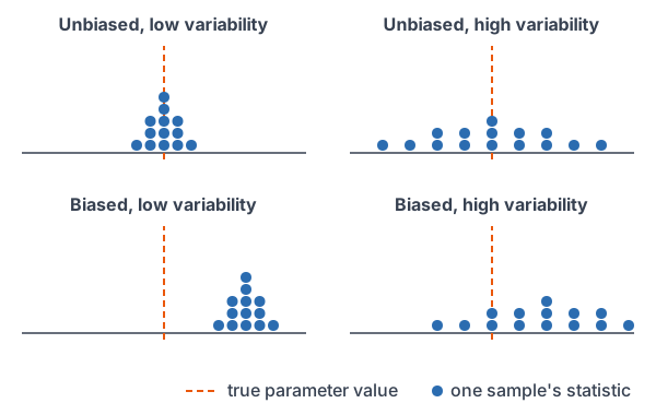
Sampling distribution examples
Example 1: Parameter or statistic?
A school has 1,200 students. Records show that 62% of all of them ride a bus. A reporter asks 50 students and finds that 58% ride a bus. Which number is a parameter and which is a statistic?
The 62% describes all 1,200 students, the whole population, so it is a parameter, p = 0.62. The 58% comes from a sample of 50 students, so it is a statistic, p̂ = 0.58.
Answer: 62% is a parameter and 58% is a statistic. The difference, 4 percentage points, is sampling variability.
Example 2: Build a sampling distribution
Example data: four roommates study 2, 4, 6 and 8 hours a week. Treat them as a population. List every sample of size 2, chosen without replacement, and find each sample mean.
\dfrac{2 + 4}{2} = \dfrac{6}{2}First sample: add the pair.
= 3
Divide by 2.
| Sample | Sample mean x̄ |
|---|---|
| 2 and 4 | 3 |
| 2 and 6 | 4 |
| 2 and 8 | 5 |
| 4 and 6 | 5 |
| 4 and 8 | 6 |
| 6 and 8 | 7 |
Answer: there are 6 samples, and their means are 3, 4, 5, 5, 6 and 7. These six values make up the sampling distribution of x̄. Each mean has probability 1/6.
Example 3: Is the sample mean unbiased?
Use Example 2. Compare the center of the sampling distribution with the population mean μ.
3 + 4 + 5 + 5 + 6 + 7 = 30
Add the six sample means.
\dfrac{30}{6} = 5Divide by 6 to find their mean.
2 + 4 + 6 + 8 = 20
Add the population values.
\mu = \dfrac{20}{4} = 5Divide by 4.
5 = 5
The center of the sampling distribution equals μ.
Answer: yes. The sample means average out to exactly μ = 5, even though no single sample is guaranteed to hit 5.
Example 4: A biased statistic
Use the same population. The population range is the largest value minus the smallest. Is the sample range an unbiased estimator of it?
2, 4, 6, 2, 4, 2
Range of each sample from Example 2: larger value minus smaller value.
2 + 4 + 6 + 2 + 4 + 2 = 20
Add the six sample ranges.
\dfrac{20}{6} \approx 3.33Divide by 6.
8 - 2 = 6
Find the population range.
3.33 \lt 6
The center is below the parameter.
Answer: no. The sample range is biased: on average it underestimates the population range, because a small sample rarely contains both extremes.
Example 5: Sample size and variability (word problem)
In a large city, 40% of adults bike to work at least once a month, so p = 0.4. Poll A samples 25 adults and Poll B samples 400. The standard deviation of p̂ is \sqrt{\dfrac{p(1 - p)}{n}} (the lesson on the sampling distribution of a sample proportion explains why). Which poll’s p̂ varies less, and by how much?
0.4(0.6) = 0.24
Find p(1 − p).
\dfrac{0.24}{25} = 0.0096Poll A: divide by n = 25.
\sqrt{0.0096} \approx 0.098Take the square root.
\dfrac{0.24}{400} = 0.0006Poll B: divide by n = 400.
\sqrt{0.0006} \approx 0.0245Take the square root.
\dfrac{0.098}{0.0245} = 4Compare the two spreads.
Answer: Poll B varies less. Its spread is about 4 times smaller, because its sample is 16 times as large. To cut the spread in half, you need 4 times as many people.
Common mistakes
| Mistake | Example of the error | Fix |
|---|---|---|
| Mixing up parameter and statistic | Calling the reporter’s 58% a parameter | A number from a sample is a statistic. |
| Thinking a bigger sample fixes bias | Trusting an online poll because 10,000 people voted | Bias comes from the method. A bigger sample only cuts variability. |
| Mixing up the three distributions | Calling a histogram of one sample’s data a sampling distribution | The sampling distribution shows a statistic from many samples. |
| Thinking unbiased means always right | Expecting x̄ = μ in every sample | Unbiased means right on average. Each x̄ still varies. |
| Using population symbols for a sample | Writing μ = 72 for the mean of 30 students | Use x̄ for a sample mean and μ for a population mean. |
Related methods
Simulating a sampling distribution
For a large population you can’t list every sample. Instead, take many random samples with a computer and plot the statistic from each one, as in probability simulations. The plot is close to the true sampling distribution.
The shape of the sampling distribution
This lesson looked at the center and spread. The next lesson, Central Limit Theorem, shows that for large samples the sampling distribution of x̄ is close to normal, whatever the population’s shape.
Practice problems
- In a survey of 200 voters, 54% favor a new park. Is 54% a parameter or a statistic? What symbol goes with it?
- The mean height of all players in a pro league is 78.5 inches. Is this a parameter or a statistic? What symbol goes with it?
- A population has the values 1, 3 and 5. List every sample of size 2 (without replacement) and its mean.
- Use Problem 3. Is the sample mean an unbiased estimator of μ?
- Use Problem 3. Find the mean of the sample maximums. Is the sample maximum an unbiased estimator of the population maximum?
- One random sample has n = 100 and another has n = 900. Which sample mean varies less, and how many times less?
- A website poll gets 20,000 votes. Is the result unbiased because the sample is so large?
- For p = 0.5 and n = 100, find the standard deviation of p̂.
- For p = 0.5 and n = 400, find the standard deviation of p̂. Compare it with Problem 8.
- An archer’s arrows land in a tight group, but the group is well to the left of the bull’s-eye. Describe the bias and variability.
Show answers
1.
The 54% comes from a sample of 200 voters.
Answer: a statistic, p̂ = 0.54
2.
The 78.5 inches describes all players in the league, the whole population.
Answer: a parameter, μ = 78.5
3.
1 + 3 = 4
Sample 1 and 3: add.
\dfrac{4}{2} = 2Divide by 2.
1 + 5 = 6
Sample 1 and 5: add.
\dfrac{6}{2} = 3Divide by 2.
3 + 5 = 8
Sample 3 and 5: add.
\dfrac{8}{2} = 4Divide by 2.
Answer: means 2, 3 and 4
4.
\dfrac{2 + 3 + 4}{3} = \dfrac{9}{3}Add the sample means.
= 3
Divide by 3.
1 + 3 + 5 = 9
Add the population values.
\mu = \dfrac{9}{3} = 3Divide by 3.
Answer: yes, both are 3
5.
3, 5, 5
Maximum of each sample.
\dfrac{3 + 5 + 5}{3} = \dfrac{13}{3}Add the maximums.
\approx 4.33
Divide by 3.
4.33 \lt 5
The population maximum is 5.
Answer: about 4.33; no, it is biased low
6.
\dfrac{900}{100} = 9The second sample is 9 times as large.
\sqrt{9} = 3The spread shrinks by the square root of that.
Answer: n = 900 varies less, about 3 times less
7.
A website poll is a voluntary response sample, so it is biased no matter how many people vote.
Answer: no
8.
0.5(0.5) = 0.25
Find p(1 − p).
\dfrac{0.25}{100} = 0.0025Divide by n.
\sqrt{0.0025} = 0.05Take the square root.
Answer: 0.05
9.
\dfrac{0.25}{400} = 0.000625Divide by n = 400.
\sqrt{0.000625} = 0.025Take the square root.
\dfrac{0.05}{0.025} = 2Compare with Problem 8.
Answer: 0.025, half as large
10.
The arrows are close together, so variability is low. Their center misses the target, so there is bias.
Answer: biased with low variability
Sampling distribution FAQ
What is a sampling distribution in statistics?
It is the distribution of a statistic, such as x̄ or p̂, from all possible samples of the same size. It shows how the statistic varies from sample to sample.
What is the difference between a parameter and a statistic?
A parameter describes a population, like μ or p. A statistic describes a sample, like x̄ or p̂, and is used to estimate the parameter.
What does unbiased mean in statistics?
A statistic is unbiased if the center of its sampling distribution equals the parameter it estimates. It is right on average, even though single samples miss.
How does sample size affect a sampling distribution?
Larger random samples make the sampling distribution less spread out. Quadrupling the sample size cuts the spread in half. Sample size does not remove bias.
Summary
- A parameter describes a population. A statistic describes a sample.
- A sampling distribution is the distribution of a statistic over all samples of the same size.
- An unbiased statistic is centered on the parameter. x̄ and p̂ are unbiased.
- Larger random samples give less variability, but they don’t fix bias.
- The best statistics are unbiased with low variability.
Previous lesson: Normal Approximation to the Binomial
Next lesson: Central Limit Theorem
Back to the Statistics Index