
Central Limit Theorem
The central limit theorem (CLT) says that when you take large random samples from any population, the sampling distribution of the sample mean x̄ is close to normal, whatever the population’s shape. Its mean is μ and its standard deviation is σ/√n. A common rule of thumb is n ≥ 30.
Before this lesson: Sampling Distributions, Standard Deviation and Normal Probability Calculations
What the central limit theorem says
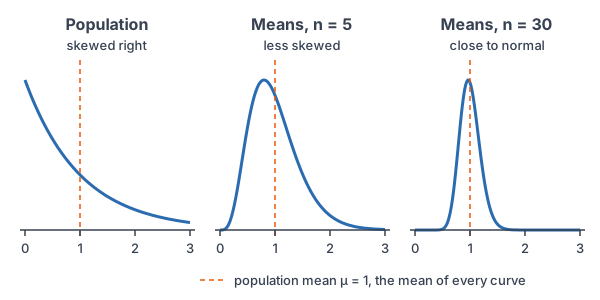
Start with a population that is not normal, such as daily phone use, which is skewed right. One person’s value can be far out in the long tail. But a sample mean averages many people. Very large and very small values tend to cancel out.
So as the sample size n grows, the distribution of x̄ gets more symmetric and more bell-shaped. It also gets narrower, because averages vary less than single values. This is true for almost any population shape.
Central limit theorem formula
\mu_{\bar{x}} = \mu \qquad \sigma_{\bar{x}} = \dfrac{\sigma}{\sqrt{n}}The mean of x̄ equals the population mean, because x̄ is unbiased. The standard deviation of x̄ is the population standard deviation divided by the square root of n. These two facts hold for any sample size. The CLT adds the shape:
- If the population is normal, x̄ is normal for any n.
- If the population is not normal, or you don’t know its shape, x̄ is approximately normal when n ≥ 30.
- If the population is strongly skewed and n is small, don’t use a normal model for x̄.
The σ/√n formula also assumes the sample is less than 10% of the population, so the values are close to independent. A later lesson, Sampling Distribution of a Sample Mean, covers that check.
Calculator: for a probability about x̄ on a TI-84, use normalcdf(lower, upper, μ, σ/√n). In Desmos, use normaldist(μ, σ/√n).cdf(a, b).
Central limit theorem examples
Example 1: Does the CLT apply?
For each case, can you use a normal model for x̄? (a) A right-skewed population with n = 50. (b) A strongly right-skewed population with n = 8. (c) A normal population with n = 5.
(a) Yes. The population is skewed, but n = 50 is at least 30, so the CLT applies. (b) No. The sample is small and the population is strongly skewed, so x̄ is still skewed. (c) Yes. When the population is normal, x̄ is exactly normal for any n.
Answer: (a) yes, by the CLT; (b) no; (c) yes, because the population is normal.
Example 2: Find the mean and standard deviation of x̄
Teens’ daily phone use has mean 4.2 hours and standard deviation 2.1 hours, and it is skewed right. A random sample of 49 teens is taken. Describe the sampling distribution of x̄.
\mu_{\bar{x}} = \mu = 4.2The mean of x̄ equals the population mean.
\sqrt{49} = 7Find the square root of n (see square roots).
\sigma_{\bar{x}} = \dfrac{2.1}{7} = 0.3Divide σ by √n.
49 \ge 30
The sample is large, so the CLT applies.
Answer: x̄ is approximately normal with mean 4.2 hours and standard deviation 0.3 hours, even though phone use itself is skewed.
Example 3: Probability for a sample mean
Use Example 2. What is the probability that the 49 teens average more than 4.7 hours a day?
z = \dfrac{4.7 - 4.2}{0.3}Change 4.7 to a z-score, using σ of x̄, not σ.
= \dfrac{0.5}{0.3}Subtract.
\approx 1.67
Divide.
P(Z \lt 1.67) = 0.9525
Read the z-table.
1 - 0.9525 = 0.0475
More than 4.7 is the right area (see complement rule).
Answer: about 0.0475. You could not find the chance that one teen uses more than 4.7 hours this way, because one teen’s value comes from the skewed population, not from a normal curve.
Example 4: Averaging dice rolls
A fair die is rolled 36 times. What is the probability that the average roll is 4 or more?
\mu = \dfrac{1 + 2 + 3 + 4 + 5 + 6}{6} = \dfrac{21}{6}Mean of one roll: add the six values.
= 3.5
Divide by 6.
\sigma = \sqrt{\dfrac{35}{12}} \approx 1.708Standard deviation of one roll (see expected value).
\sigma_{\bar{x}} = \dfrac{1.708}{\sqrt{36}} = \dfrac{1.708}{6}Use n = 36, so √n = 6.
\approx 0.2847
Divide.
z = \dfrac{4 - 3.5}{0.2847} = \dfrac{0.5}{0.2847}Change 4 to a z-score: subtract.
\approx 1.76
Divide.
1 - 0.9608 = 0.0392
P(Z \lt 1.76) = 0.9608, so take the right area.
Answer: about 0.0392. One roll is uniform, not normal, but the mean of 36 rolls is close to normal.
Example 5: Elevator capacity (word problem)
An elevator has a limit of 3,800 pounds and holds 20 people. Adult weights are approximately normal with mean 180 pounds and standard deviation 35 pounds. If 20 random adults get on, what is the probability that they are over the limit?
\dfrac{3800}{20} = 190Over the limit means the mean weight is over 190 pounds.
\sqrt{20} \approx 4.472Find √n.
\sigma_{\bar{x}} = \dfrac{35}{4.472} \approx 7.826Divide σ by √n.
z = \dfrac{190 - 180}{7.826} = \dfrac{10}{7.826}Change 190 to a z-score: subtract.
\approx 1.28
Divide.
1 - 0.8997 = 0.1003
P(Z \lt 1.28) = 0.8997, so take the right area.
Answer: about 0.10. Here n = 20 is less than 30, but that is fine because the population of weights is approximately normal.
Common mistakes
| Mistake | Example of the error | Fix |
|---|---|---|
| Using σ instead of σ/√n | z = (4.7 − 4.2)/2.1 for a sample mean | For x̄, divide by σ/√n = 0.3. |
| Dividing by n instead of √n | σ of x̄ = 2.1/49 | Divide by √49 = 7. |
| Saying the population becomes normal | With n = 49, phone use is normal | Only the distribution of x̄ becomes normal. The population keeps its shape. |
| Using the CLT for one individual | Finding P(one teen uses more than 4.7 hours) from the z-table | One value comes from the skewed population, so a normal model doesn’t fit. |
| Using a normal model for a small skewed sample | A normal model for x̄ with n = 8 from skewed data | Use n ≥ 30, or a normal population. |
Related methods
Sums and counts
The CLT also covers sums, since a sum is just n times the mean. That is why a binomial count, a sum of many 0s and 1s, is close to normal for large n (see normal approximation to the binomial). Rules for the mean and spread of sums come from combining random variables.
Why the CLT matters
Confidence intervals and hypothesis tests for means rely on x̄ being close to normal. The CLT is what makes them work even when the population isn’t normal.
Practice problems
- A population is skewed left, and n = 60. Can you use a normal model for x̄?
- A population is strongly skewed right, and n = 10. Can you use a normal model for x̄?
- A population is normal, and n = 4. Can you use a normal model for x̄?
- A population has μ = 50 and σ = 12. For n = 36, find the mean and standard deviation of x̄.
- Use Problem 4. Find P(\bar{x} \lt 47).
- Use Problem 4. Find P(48 \lt \bar{x} \lt 53).
- With σ = 12, how large must n be for the standard deviation of x̄ to equal 1?
- Use Example 4. Find the probability that the average of 36 rolls is 3 or less.
- Delivery times have mean 32 minutes and standard deviation 10 minutes, and they are skewed right. For 40 random deliveries, find P(\bar{x} \gt 35).
- Use Problem 9. Why can’t you use the z-table to find the probability that one delivery takes more than 35 minutes?
Show answers
1.
The population is skewed, but n = 60 is at least 30.
Answer: yes, by the CLT
2.
The sample is small, and the population is strongly skewed.
Answer: no
3.
When the population is normal, x̄ is normal for any n.
Answer: yes
4.
\mu_{\bar{x}} = 50Same as the population mean.
\sqrt{36} = 6Find √n.
\sigma_{\bar{x}} = \dfrac{12}{6} = 2Divide σ by √n.
Answer: mean 50, standard deviation 2
5.
z = \dfrac{47 - 50}{2} = \dfrac{-3}{2}Change 47 to a z-score: subtract.
= -1.5
Divide.
P(Z \lt -1.5) = 0.0668
Read the z-table.
Answer: about 0.0668
6.
z = \dfrac{48 - 50}{2} = \dfrac{-2}{2}Lower z: subtract.
= -1
Divide.
z = \dfrac{53 - 50}{2} = \dfrac{3}{2}Upper z: subtract.
= 1.5
Divide.
0.9332 - 0.1587 = 0.7745
Subtract the left areas.
Answer: about 0.7745
7.
\dfrac{12}{\sqrt{n}} = 1Set the standard deviation of x̄ equal to 1.
\sqrt{n} = 12Multiply both sides by √n.
n = 144
Square both sides.
Answer: n = 144
8.
z = \dfrac{3 - 3.5}{0.2847} = \dfrac{-0.5}{0.2847}Change 3 to a z-score: subtract.
\approx -1.76
Divide.
P(Z \lt -1.76) = 0.0392
Read the z-table.
Answer: about 0.0392
9.
\sqrt{40} \approx 6.325Find √n.
\sigma_{\bar{x}} = \dfrac{10}{6.325} \approx 1.581Divide σ by √n.
z = \dfrac{35 - 32}{1.581} = \dfrac{3}{1.581}Change 35 to a z-score: subtract.
\approx 1.90
Divide.
1 - 0.9713 = 0.0287
P(Z \lt 1.90) = 0.9713, so take the right area.
Answer: about 0.0287
10.
One delivery time comes from the population, which is skewed right, so it doesn’t follow a normal curve. The CLT is about x̄, not single values.
Answer: the population isn’t normal
Central limit theorem FAQ
What does the central limit theorem say?
For large random samples, the sampling distribution of the sample mean is approximately normal, with mean μ and standard deviation σ/√n, no matter what shape the population has.
Why is n ≥ 30 used for the central limit theorem?
It is a rule of thumb. For most populations, samples of 30 or more give a sampling distribution of x̄ that is close enough to normal. Very skewed populations may need larger samples.
Does the central limit theorem make the data normal?
No. The population and the data in each sample keep their shape. Only the distribution of the sample mean becomes close to normal.
Why is the central limit theorem important?
It lets you use normal calculations for sample means from almost any population. Confidence intervals and hypothesis tests depend on it.
Summary
- The mean of x̄ is μ, and its standard deviation is σ/√n.
- If the population is normal, x̄ is normal for any n.
- Otherwise, x̄ is approximately normal when n ≥ 30.
- Use σ/√n, not σ, in z-scores for x̄.
- The CLT is about sample means, not single values or the population.
Previous lesson: Sampling Distributions
Next lesson: Sampling Distribution of a Sample Proportion
Back to the Statistics Index