
Normal Probability Calculations
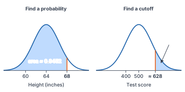
Normal probability calculations answer two questions about a normal distribution: what is the probability that a value falls in a range, and what value cuts off a given percent? For a normal distribution probability, change each value to a z-score and use a z-table or a calculator. For a cutoff, work backward.
Before this lesson: Normal Distribution, Standard Normal Distribution and Percentiles and Z-Scores
The idea: turn any normal curve into the standard one
A probability for a normal variable is an area under its curve, just like on any density curve. The z-table only covers N(0, 1). So you change each value x into a z-score, which counts standard deviations from the mean. The area to the left of x is the same as the area to the left of its z-score.
z = \dfrac{x - \mu}{\sigma} \qquad x = \mu + z\sigmaUse the first formula to find a probability. Use the second one, solved for x, to find a cutoff value.
How to find a normal distribution probability
- Draw the curve, mark the mean, and shade the area you want.
- Change each value to a z-score.
- Find the area with the z-table or a calculator. Subtract from 1 for a right area.
- Answer the question in context.
How to find a cutoff value
- Shade the area you know. Find the area to the left of the cutoff.
- Find the z-score for that left area in the z-table, or use invNorm.
- Change z back to x with x = \mu + z\sigma.
- Answer the question in context.
z-scores used in this lesson
| z | Area to the left | z | Area to the left |
|---|---|---|---|
| −2.50 | 0.0062 | 0.67 | 0.7486 |
| −2.33 | 0.0099 | 0.68 | 0.7517 |
| −2.00 | 0.0228 | 0.80 | 0.7881 |
| −1.60 | 0.0548 | 1.20 | 0.8849 |
| −1.25 | 0.1056 | 1.25 | 0.8944 |
| −1.20 | 0.1151 | 1.28 | 0.8997 |
| −0.84 | 0.2005 | 1.50 | 0.9332 |
| 2.00 | 0.9772 | 1.60 | 0.9452 |
Calculator: on a TI-84, normalcdf(lower, upper, μ, σ) finds an area without a z-score, and invNorm(left area, μ, σ) finds a cutoff. Both are under 2nd, VARS (DISTR). In Desmos, normaldist(μ, σ).cdf(a, b) gives the area between a and b. Many teachers still want the z-score work, so show it first.
Normal probability examples
Example 1: Probability less than a value
Women’s heights are approximately normal with mean 64 inches and standard deviation 2.5 inches. What proportion of women are shorter than 68 inches?
z = \dfrac{68 - 64}{2.5}Change 68 to a z-score.
= \dfrac{4}{2.5}Subtract.
= 1.6
Divide (see dividing decimals).
P(X \lt 68) = P(Z \lt 1.6)
The area to the left of 68 equals the area to the left of z = 1.6.
= 0.9452
Read the z-table.
Answer: about 0.9452, so about 94.5% of women are shorter than 68 inches. Calculator check: normalcdf(−1E99, 68, 64, 2.5) ≈ 0.9452. In Desmos, normaldist(64, 2.5).cdf(68) gives the same value.
Example 2: Probability greater than a value
Scores on a college entrance test are approximately normal with mean 500 and standard deviation 100. What proportion of scores are above 650?
z = \dfrac{650 - 500}{100}Change 650 to a z-score.
= \dfrac{150}{100}Subtract.
= 1.5
Divide.
P(Z \lt 1.5) = 0.9332
Read the z-table.
P(X \gt 650) = 1 - 0.9332
Above 650 is the right area (see complement rule).
= 0.0668
Subtract.
Answer: about 0.0668, or 6.68% of scores. With a calculator, normalcdf(650, 1E99, 500, 100) ≈ 0.0668.
Example 3: Probability between two values
Car battery lifetimes are approximately normal with mean 4.5 years and standard deviation 0.8 years. What is the probability that a battery lasts between 3.5 and 5.5 years?
z_1 = \dfrac{3.5 - 4.5}{0.8}Change the lower value to a z-score.
= \dfrac{-1}{0.8}Subtract.
= -1.25
Divide. A negative divided by a positive is negative (see dividing signed numbers).
z_2 = \dfrac{5.5 - 4.5}{0.8}Change the upper value to a z-score.
= \dfrac{1}{0.8}Subtract.
= 1.25
Divide.
P(-1.25 \lt Z \lt 1.25) = 0.8944 - 0.1056
Left area at 1.25 minus left area at −1.25.
= 0.7888
Subtract.
Answer: about 0.7888. A calculator gives normalcdf(3.5, 5.5, 4.5, 0.8) ≈ 0.7887. The last digit differs because the table rounds each area.
Example 4: Find a cutoff for the top 10%
Use the test scores from Example 2. A scholarship goes to the top 10% of scores. What is the lowest score that qualifies?
1 - 0.10 = 0.90
The top 10% has 90% of the area to its left.
z \approx 1.28
The closest table area to 0.90 is 0.8997, at z = 1.28.
x = 500 + 1.28(100)
Change z back to x with x = μ + zσ.
= 500 + 128
Multiply.
= 628
Add.
Answer: a score of about 628 or higher qualifies. On a TI-84, invNorm(0.90, 500, 100) ≈ 628.16.
Example 5: Filling cereal boxes (word problem)
A machine fills cereal boxes labeled 500 grams. The fill weights are approximately normal with mean 510 grams and standard deviation 4 grams. (a) What proportion of boxes are underweight? (b) The company wants only 1% of boxes underweight. If σ stays at 4 grams, what mean fill should it set?
z = \dfrac{500 - 510}{4}(a) Change 500 to a z-score.
= \dfrac{-10}{4}Subtract.
= -2.5
Divide.
P(X \lt 500) = 0.0062
Read the table at z = −2.50.
z \approx -2.33
(b) The left area should be 0.01. The closest table area is 0.0099, at z = −2.33.
500 = \mu + (-2.33)(4)
The label weight must be 2.33 standard deviations below the new mean.
500 = \mu - 9.32
Multiply.
509.32 = \mu
Add 9.32 to both sides.
Answer: (a) about 0.0062, or 0.62% of boxes; (b) a mean fill of about 509.3 grams. With invNorm, the mean comes out to about 509.31 grams.
Common mistakes
| Mistake | Example of the error | Fix |
|---|---|---|
| Looking up the raw value | Looking up 68 in the z-table | Find z first: (68 − 64)/2.5 = 1.6. |
| Dividing by the variance | z = (68 − 64)/6.25 | Divide by σ = 2.5, not by σ². |
| Subtracting in the wrong order | z = (64 − 68)/2.5 = −1.6 | Always use value minus mean: (x − μ)/σ. |
| Using a left area for “more than” | P(X > 650) = 0.9332 | Subtract from 1: 0.0668. |
| Giving the area as the cutoff | Saying the top 10% starts at 0.90 | Change the area to z, then z to x: 628. |
| Using the right area in invNorm | invNorm(0.10, 500, 100) for the top 10% | invNorm uses the left area: invNorm(0.90, 500, 100). |
Related methods
Check with the empirical rule
Before you trust an answer, compare it with the empirical rule. In Example 2, 650 is 1.5σ above the mean. That is between 1σ (16% above) and 2σ (2.5% above), so 6.68% is reasonable.
Is the distribution close to normal?
These steps only work for a distribution that is close to normal. For data, check the shape first. The next lesson, Normal Probability Plots, shows how.
Practice problems
Use the table above or a calculator. Women’s heights are N(64, 2.5) inches, test scores are N(500, 100), and battery lifetimes are N(4.5, 0.8) years.
- What proportion of women are shorter than 60 inches?
- What proportion of women are taller than 66 inches?
- What proportion of women are between 61 and 67 inches tall?
- What proportion of test scores are below 380?
- What test score is at the 75th percentile?
- What proportion of batteries last more than 6.1 years?
- A store wants only 5% of batteries to fail before the warranty ends. How long should the warranty be?
- What height separates the shortest 20% of women from the rest?
- Cereal fills are N(510, 4) grams. What proportion of boxes hold more than 515 grams?
- Bolt lengths are N(30, 0.2) mm. Bolts from 29.6 to 30.4 mm pass inspection. What proportion fail?
Show answers
1.
z = \dfrac{60 - 64}{2.5}Change 60 to a z-score.
= \dfrac{-4}{2.5}Subtract.
= -1.6
Divide.
P(Z \lt -1.6) = 0.0548
Read the table.
Answer: about 0.0548
2.
z = \dfrac{66 - 64}{2.5}Change 66 to a z-score.
= \dfrac{2}{2.5}Subtract.
= 0.8
Divide.
1 - 0.7881 = 0.2119
Taller means the right area.
Answer: about 0.2119
3.
z_1 = \dfrac{61 - 64}{2.5} = \dfrac{-3}{2.5}Lower value: subtract.
= -1.2
Divide.
z_2 = \dfrac{67 - 64}{2.5} = \dfrac{3}{2.5}Upper value: subtract.
= 1.2
Divide.
0.8849 - 0.1151 = 0.7698
Subtract the left areas.
Answer: about 0.7698
4.
z = \dfrac{380 - 500}{100}Change 380 to a z-score.
= \dfrac{-120}{100}Subtract.
= -1.2
Divide.
P(Z \lt -1.2) = 0.1151
Read the table.
Answer: about 0.1151
5.
z \approx 0.67
0.7486 (at 0.67) is closer to 0.75 than 0.7517 (at 0.68).
x = 500 + 0.67(100)
Use x = μ + zσ.
= 500 + 67
Multiply.
= 567
Add.
Answer: about 567 (invNorm gives 567.45)
6.
z = \dfrac{6.1 - 4.5}{0.8}Change 6.1 to a z-score.
= \dfrac{1.6}{0.8}Subtract.
= 2
Divide.
1 - 0.9772 = 0.0228
More than means the right area.
Answer: about 0.0228
7.
z \approx -1.645
The left area is 0.05. By symmetry with the top 5%, z ≈ −1.645.
x = 4.5 + (-1.645)(0.8)
Use x = μ + zσ.
= 4.5 - 1.316
Multiply.
= 3.184
Subtract.
Answer: about 3.2 years
8.
z \approx -0.84
The closest table area to 0.20 is 0.2005, at z = −0.84.
x = 64 + (-0.84)(2.5)
Use x = μ + zσ.
= 64 - 2.1
Multiply.
= 61.9
Subtract.
Answer: about 61.9 inches
9.
z = \dfrac{515 - 510}{4}Change 515 to a z-score.
= \dfrac{5}{4}Subtract.
= 1.25
Divide.
1 - 0.8944 = 0.1056
More than means the right area.
Answer: about 0.1056
10.
z = \dfrac{29.6 - 30}{0.2} = \dfrac{-0.4}{0.2}Lower limit: subtract.
= -2
Divide.
z = \dfrac{30.4 - 30}{0.2} = \dfrac{0.4}{0.2}Upper limit: subtract.
= 2
Divide.
0.9772 - 0.0228 = 0.9544
Proportion that pass.
1 - 0.9544 = 0.0456
Proportion that fail.
Answer: about 0.0456
Normal distribution probability FAQ
How do you find a probability in a normal distribution?
Change the value to a z-score with z = (x − μ)/σ. Then find the area to the left of z in a z-table, and subtract from 1 if you need the area to the right.
How do you find a value from a percentile in a normal distribution?
Find the z-score with that percent of the area to its left, then use x = μ + zσ. On a TI-84, invNorm(percent, μ, σ) does both steps.
What does normalcdf do on a TI-84?
It finds the area under a normal curve between a lower and an upper bound. Enter the bounds, then the mean and standard deviation.
Why do the table and the calculator give slightly different answers?
The table rounds z to two decimal places and each area to four. The calculator does not round, so the last digit can differ.
Summary
- To find a probability, change x to z = (x − μ)/σ, then use the z-table.
- Subtract from 1 for a right area. Subtract two left areas for an area between.
- To find a cutoff, get z from the left area, then use x = μ + zσ.
- On a TI-84, normalcdf finds areas and invNorm finds cutoffs. invNorm always uses the left area.
- Check that your answer makes sense with the empirical rule.
Previous lesson: Standard Normal Distribution
Next lesson: Normal Probability Plots
Back to the Statistics Index