
Probability Rules
The basic probability rules say that every probability is between 0 and 1, the probabilities of all outcomes in the sample space add to 1, and the probability that an event does not happen is 1 minus the probability that it does. The law of large numbers says long-run relative frequencies settle near the true probability.
Before this lesson: Probability, Fractions and Probability Simulations
Sample spaces and events
A random process has outcomes we can’t predict one at a time, like flipping a coin. The sample space, written S, is the list of all possible outcomes. An event is any set of outcomes, and it is usually named with a capital letter like A.
For one roll of a die, the sample space is S = \{1, 2, 3, 4, 5, 6\}. The event “roll an even number” is A = \{2, 4, 6\}.
When all outcomes are equally likely, the probability of an event is the number of outcomes in the event divided by the number of outcomes in the sample space. So P(A) = \frac{3}{6} = \frac{1}{2}.
The basic probability rules
0 \le P(A) \le 1
Rule 1: every probability is between 0 and 1. A probability of 0 means the event never happens, and 1 means it always happens.
P(S) = 1
Rule 2: the probabilities of all the outcomes in the sample space add to 1. Something in the sample space must happen.
P(A^C) = 1 - P(A)
Rule 3, the complement rule: the complement of A, written A^C, is the event that A does not happen. Its probability is 1 minus the probability of A. This rule is the fastest way to handle “at least one” questions.
A list of outcomes with their probabilities is called a probability model. A model is valid only if every probability is between 0 and 1 and they all add to 1.
The law of large numbers
The law of large numbers says that as a random process is repeated many times, the relative frequency of an event (the share of trials where it happens) gets closer to its true probability. This is why simulations with many trials work.
The law is about the long run only. Over a few trials, results can stray far from the probability, and earlier results don’t change the next one. A coin that just landed heads 5 times is still 50-50 on the next flip.
Probability rules examples
Example 1: Use a sample space
A coin is flipped 3 times. Find the probability of getting exactly 2 heads.
2 \times 2 \times 2 = 8
Each flip has 2 outcomes, so multiply to count the sample space.
\text{HHH, HHT, HTH, HTT, THH, THT, TTH, TTT}List the 8 equally likely outcomes.
\text{HHT, HTH, THH}Pick out the outcomes with exactly 2 heads.
P(\text{2 heads}) = \dfrac{3}{8}Divide the 3 outcomes by the 8 in the sample space.
\dfrac{3}{8} = 0.375Write as a decimal.
Answer: the probability is 3/8, or 0.375.
Example 2: Complete a probability model
A school asks students to pick their favorite lunch (example data). Pizza has probability 0.38, tacos 0.27 and salad 0.14. Burgers are the only other choice. Find the probability that a random student picks burgers.
0.38 + 0.27 + 0.14 = 0.79
Add the known probabilities.
1 - 0.79 = 0.21
Rule 2: all probabilities add to 1, so subtract from 1.
0 \le 0.21 \le 1
Rule 1: check that the answer is a valid probability.
Answer: P(burgers) = 0.21.
Example 3: Use the complement rule with two dice
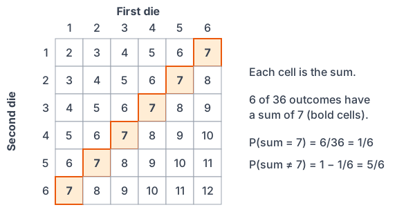
Two fair dice are rolled. Find the probability that the sum is not 7.
6 \times 6 = 36
Count the outcomes: 6 for the first die times 6 for the second.
(1,6), (2,5), (3,4), (4,3), (5,2), (6,1)
List the outcomes with a sum of 7.
P(\text{sum } 7) = \dfrac{6}{36}Divide 6 outcomes by 36.
\dfrac{6}{36} = \dfrac{1}{6}Simplify the fraction (see fractions).
P(\text{not } 7) = 1 - \dfrac{1}{6}Use the complement rule.
1 - \dfrac{1}{6} = \dfrac{5}{6}Subtract: 1 is the same as 6/6.
Answer: the probability that the sum is not 7 is 5/6, or about 0.833. Counting the 30 outcomes that are not 7 gives the same answer, but the complement is faster.
Example 4: An “at least one” question
A coin is flipped 4 times. Find the probability of at least one head.
2^4 = 16
Count the outcomes in the sample space (see exponents).
\text{TTTT}The complement, “no heads,” has only this one outcome.
P(\text{no heads}) = \dfrac{1}{16}One outcome out of 16.
P(\text{at least one head}) = 1 - \dfrac{1}{16}Use the complement rule.
1 - \dfrac{1}{16} = \dfrac{15}{16}Subtract: 1 is the same as 16/16.
\dfrac{15}{16} = 0.9375Write as a decimal.
Answer: 15/16, or 0.9375. “At least one” includes 1, 2, 3 or 4 heads, so the single outcome with none is much easier to count.
Example 5: The law of large numbers (word problem)
A factory says 2% of its light bulbs are defective. An inspector keeps a running count (example data): 3 defective in the first 50 bulbs, 13 in the first 500 and 104 in the first 5,000. Find the relative frequency at each point and explain the pattern.
\dfrac{3}{50} = 0.06Relative frequency after 50 bulbs.
\dfrac{13}{500} = 0.026Relative frequency after 500 bulbs.
\dfrac{104}{5000} = 0.0208Relative frequency after 5,000 bulbs.
0.0208 - 0.02 = 0.0008
Compare the last value with the claimed 0.02.
Answer: 6%, then 2.6%, then 2.08%. The early count was high just by chance, and the relative frequency moved closer to 2% as the count grew. That is the law of large numbers at work.
Common mistakes
| Mistake | Example of the error | Fix |
|---|---|---|
| A model that doesn’t add to 1 | Giving outcomes the probabilities 0.3, 0.5 and 0.25 | Check that the probabilities add to exactly 1 (these add to 1.05). |
| Thinking chance “evens out” soon | “After 5 heads, tails is due.” | Each flip is still 50-50. The law of large numbers is about the long run only. |
| Wrong complement for “at least one” | Using “all heads” as the complement of “at least one head” | The complement of “at least one” is “none.” |
| Counting outcomes that aren’t equally likely | Saying the sums 2 to 12 are 11 outcomes, so P(7) = 1/11 | Use the 36 equally likely ordered pairs, so P(7) = 6/36. |
| Treating (1, 6) and (6, 1) as the same | Listing only 3 ways to roll a sum of 7 | With two dice, order matters: there are 6 ways. |
| Probabilities outside 0 to 1 | Writing P(A) = 1.2 or P(A) = 120 | Every probability is between 0 and 1. Write 12% as 0.12. |
Related methods
Counting larger sample spaces
When listing every outcome takes too long, multiply the number of choices at each step, as in Examples 1 and 4. For choosing groups, use permutations and combinations.
Probabilities from data
Probabilities can also come from data, such as a relative frequency from a survey or a two-way table. When a probability is hard to count, a probability simulation estimates it, and the law of large numbers says more trials give a better estimate.
Practice problems
- A spinner has 3 equal sections: red, blue and green. It is spun twice. How many outcomes are in the sample space, and what is the probability of the same color both times?
- Is this a valid probability model: P(A) = 0.3, P(B) = 0.5, P(C) = 0.25? Explain.
- A model has four outcomes. Three have probabilities 0.12, 0.35 and 0.28. Find the fourth.
- The chance of rain tomorrow is 0.65. What is the chance of no rain?
- Two dice are rolled. Find the probability of doubles and the probability of not getting doubles.
- A coin is flipped 3 times. Find the probability of at least one tail.
- One card is drawn from a standard 52-card deck, which has 13 hearts. Find the probability that it is not a heart.
- A coin lands heads 7 times in 10 flips. Is the next flip more likely to be tails? Explain.
- A die is rolled 1,000 times and lands on 6 a total of 171 times. Find the relative frequency and compare it with the true probability.
- Which of these can be probabilities: 0, 0.99, 1.2, −0.1, 3/4?
Show answers
1.
3 \times 3 = 9
Multiply 3 colors for each spin.
\text{RR, BB, GG}List the outcomes with the same color.
\dfrac{3}{9} = \dfrac{1}{3}Divide and simplify.
Answer: 9 outcomes; the probability is 1/3
2.
0.3 + 0.5 + 0.25 = 1.05
Add the probabilities.
Answer: no, because the probabilities add to 1.05, not 1
3.
0.12 + 0.35 + 0.28 = 0.75
Add the known probabilities.
1 - 0.75 = 0.25
Subtract from 1.
Answer: 0.25
4.
1 - 0.65 = 0.35
Use the complement rule.
Answer: 0.35
5.
\dfrac{6}{36} = \dfrac{1}{6}There are 6 doubles out of 36 outcomes.
1 - \dfrac{1}{6} = \dfrac{5}{6}Use the complement rule.
Answer: P(doubles) = 1/6; P(not doubles) = 5/6
6.
2^3 = 8
Count the outcomes.
P(\text{no tails}) = \dfrac{1}{8}Only HHH has no tails.
1 - \dfrac{1}{8} = \dfrac{7}{8}Use the complement rule.
Answer: 7/8, or 0.875
7.
P(\text{heart}) = \dfrac{13}{52} = \dfrac{1}{4}Divide and simplify.
1 - \dfrac{1}{4} = \dfrac{3}{4}Use the complement rule.
Answer: 3/4, or 0.75
8.
\text{each flip: } P(\text{tails}) = \dfrac{1}{2}The coin has no memory.
Answer: no; the next flip is still 50-50, because the law of large numbers only describes the long run
9.
\dfrac{171}{1000} = 0.171Find the relative frequency.
\dfrac{1}{6} \approx 0.167Find the true probability.
Answer: 0.171, close to the true probability of about 0.167
10.
0 \le P \le 1
A probability must be between 0 and 1.
Answer: 0, 0.99 and 3/4 can be probabilities; 1.2 and −0.1 cannot
Probability rules FAQ
What are the basic rules of probability?
Every probability is between 0 and 1, the probabilities of all outcomes in the sample space add to 1, and the probability that an event does not happen is 1 minus the probability that it does.
What is the complement rule in probability?
It says P(A^C) = 1 - P(A). For example, if the chance of rain is 0.3, the chance of no rain is 0.7.
What is a sample space?
The sample space is the list of every possible outcome of a random process. For one die it is 1, 2, 3, 4, 5 and 6.
What does the law of large numbers say?
As a random process is repeated many times, the share of times an event happens gets closer to its true probability. It says nothing about the next single trial.
Summary
- The sample space S lists all outcomes. An event is a set of outcomes.
- With equally likely outcomes, P(A) = outcomes in A divided by outcomes in S.
- Every probability is between 0 and 1, and the probabilities of all outcomes add to 1.
- Complement rule: P(A^C) = 1 - P(A). Use it for “at least one” questions.
- Law of large numbers: in the long run, relative frequency gets close to the true probability.
Previous lesson: Probability Simulations
Next lesson: Addition Rule and Mutually Exclusive Events
Back to the Statistics Index