Normal Probability Plot: How to Read One

A normal probability plot is a graph that shows whether a data set is close to normal. Each data value is plotted against the z-score it would have in a perfectly normal data set of the same size. If the points fall close to a straight line, the data are close to normal.

Before this lesson: Describing a Distribution, Normal Distribution and Normal Probability Calculations

Why the plot works

Picture a perfectly normal data set with 10 values. Its smallest value would sit about 1.64 standard deviations below the mean. The next would sit about 1.04 below, and so on. These are the expected z-scores.

If the data are normal, each value is close to μ + zσ. That is a linear equation in z, so the points line up. If the data are skewed or have outliers, the points bend away from a line.

How to make a normal probability plot

Sort the data from smallest to largest. Number the values i = 1, 2, 3 and so on, up to n.
Find each value’s percentile: $p = \dfrac{i - 0.5}{n}$ .
Find the z-score with that much area to its left, with a z-table or invNorm(p, 0, 1).
Plot each point with the data value across and its z-score up the side.

Some books and calculators use a slightly different percentile formula or swap the axes. The plot is read the same way.

Calculator: on a TI-84, put the data in L1. Press 2nd, Y= (STAT PLOT), turn Plot 1 on, and choose the last plot type, the normal probability plot. Set Data List to L1 and Data Axis to X, then press ZOOM, 9. Desmos has no built-in normal probability plot, so type the data values and their z-scores into a table and plot the pairs.

How to read a normal probability plot

Pattern	What it means
Points close to a straight line	The data are close to normal.
Steep at the left, then flatter at the right	Skewed right: the large values are spread far apart.
Flat at the left, then steeper at the right	Skewed left: the small values are spread far apart.
One point far from the line at an end	An outlier.
A few small wiggles around the line	Still close to normal. Small samples are never perfectly straight.

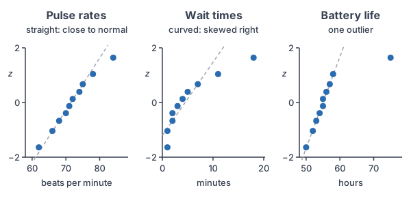
Left: the points lie near the line, so the pulse rates are close to normal. Middle: the curve shows right skew. Right: one point is an outlier.

Normal probability plot examples

Example 1: Find the expected z-scores

Example data: the resting pulse rates of 10 students, in beats per minute, sorted from smallest to largest: 62, 66, 68, 70, 71, 72, 74, 75, 78, 84. Find the percentile and z-score for the smallest and largest values, then list all ten z-scores.

p_1 = \dfrac{1 - 0.5}{10}

The smallest value has i = 1.

= \dfrac{0.5}{10}

Subtract.

= 0.05

Divide.

z_1 \approx -1.64

invNorm(0.05, 0, 1) ≈ −1.6449, about −1.64.

p_{10} = \dfrac{10 - 0.5}{10}

The largest value has i = 10.

= \dfrac{9.5}{10}

Subtract.

= 0.95

Divide.

z_{10} \approx 1.64

By symmetry, it is the opposite of z₁.

i	Pulse	p	Expected z
1	62	0.05	−1.64
2	66	0.15	−1.04
3	68	0.25	−0.67
4	70	0.35	−0.39
5	71	0.45	−0.13
6	72	0.55	0.13
7	74	0.65	0.39
8	75	0.75	0.67
9	78	0.85	1.04
10	84	0.95	1.64

Answer: the z-scores run from −1.64 to 1.64 and are symmetric about 0. The left panel of the graph above plots these ten pairs.

Example 2: Read a plot that is close to a line

Use the left panel of the graph. Are the pulse rates close to normal?

The points rise from lower left to upper right in a nearly straight line. There is no clear bend, and no point is far from the line. The point at 84 is a little to the right, but one small wiggle in 10 values is expected.

Answer: yes, the pulse rates are close to normal, so normal calculations are reasonable for them.

Example 3: Read a curved plot

Example data: wait times at a coffee shop, in minutes: 1, 1, 2, 2, 3, 4, 5, 7, 11, 18. With n = 10, the expected z-scores are the same as in Example 1. Use the middle panel. Describe the shape.

-1.04 - (-1.64) = 0.60

The two smallest values are 0.60 apart in z.

1 - 1 = 0

But they are 0 minutes apart, so the plot is steep at the left.

1.64 - 1.04 = 0.60

The two largest values are also 0.60 apart in z.

18 - 11 = 7

But they are 7 minutes apart, so the plot is flat at the right.

Answer: the plot is steep at the left and flat at the right, so it curves. The wait times are skewed right, not normal. Don’t use normal calculations for them.

Example 4: Spot an outlier

Example data: battery life of 10 phones, in hours: 50, 52, 53, 54, 55, 55, 56, 57, 58, 75. Use the right panel. Is any value an outlier?

58 - 50 = 8

The first nine values span only 8 hours, and they line up.

75 - 58 = 17

The largest value is 17 hours past the next one, far right of the line.

\text{IQR} = 57 - 53 = 4

Check with the 1.5 × IQR rule: Q1 = 53 and Q3 = 57 (see outliers).

57 + 1.5(4) = 57 + 6

Upper fence: multiply.

= 63

Add.

75 \gt 63

75 is above the fence, so it is an outlier.

Answer: 75 hours is an outlier, so the data as a whole are not close to normal. Check that value for a mistake before you go on.

Example 5: Check the plot, then use a normal model (word problem)

The plot in Example 2 shows the pulse rates are close to normal. Use the sample mean and standard deviation to estimate the percent of students with a resting pulse above 80.

62 + 66 + 68 + 70 + 71 + 72 + 74 + 75 + 78 + 84 = 720

Add the data.

\bar{x} = \dfrac{720}{10} = 72

Divide by n = 10 to get the mean.

100 + 36 + 16 + 4 + 1 + 0 + 4 + 9 + 36 + 144 = 350

Square each deviation from 72 and add them (see standard deviation).

\dfrac{350}{9} \approx 38.89

Divide by n − 1 = 9 to get the variance.

s = \sqrt{38.89} \approx 6.24

Take the square root.

z = \dfrac{80 - 72}{6.24}

Change 80 to a z-score.

= \dfrac{8}{6.24}

Subtract.

\approx 1.28

Divide.

1 - 0.8997 = 0.1003

Above 80 is the right area. The table gives 0.8997 at z = 1.28.

Answer: about 10% of students. On a TI-84, 1-Var Stats gives a mean of 72 and Sx ≈ 6.24, and normalcdf(80, 1E99, 72, 6.24) ≈ 0.10.

Common mistakes

Mistake	Example of the error	Fix
Expecting a perfect line	Calling the pulse data not normal because of one small wiggle	Look for a clear curve or an outlier, not small wiggles.
Forgetting to sort	Pairing the first value listed with z = −1.64	Sort the data from smallest to largest first.
Using i/n for the percentile	p = 10/10 = 1 for the largest value	Use (i − 0.5)/n. No z-score has an area of 1 to its left.
Calling a curved plot normal	Using normal calculations for the wait times	A clear bend means skew, so the data are not close to normal.
Ignoring an outlier	Using normal calculations for the battery data	Check the outlier first. With it, the data are not close to normal.
Mixing up the axes	Reading the z-scores as data values	Check which axis holds the data and which holds z.

Related methods

Other ways to check the shape

A histogram or a box plot also shows skew and outliers. If the mean and the median are far apart, the data are probably skewed. The normal probability plot is the most sensitive check, especially for small data sets.

Normal shapes in other distributions

Some counts, like the number of successes in many trials, have a binomial distribution that is close to normal. The next lesson, Normal Approximation to the Binomial, uses that.

Practice problems

A data set has n = 8 values. Find the percentile p for the smallest value.
A data set has n = 8 values. Find p for the largest value.
Use a calculator to find the expected z-score for p = 0.0625.
A normal probability plot is close to a straight line. What does that tell you?
A plot is steep at the left and flattens out at the right. What is the shape of the data?
All points line up except the smallest one, which is far to the left of the line. What does that show?
A data set has n = 5 values. Find p and the expected z-score for each position.
Why do we use (i − 0.5)/n and not i/n for the percentile?
Use the pulse data from Example 5, with mean 72 and s = 6.24. Estimate the percent of students with a pulse below 65.
Is it reasonable to use a normal model for the coffee shop wait times in Example 3? Explain.

Show answers

p = \dfrac{1 - 0.5}{8}

Use i = 1 and n = 8.

= \dfrac{0.5}{8}

Subtract.

= 0.0625

Divide.

Answer: 0.0625

p = \dfrac{8 - 0.5}{8}

Use i = 8 and n = 8.

= \dfrac{7.5}{8}

Subtract.

= 0.9375

Divide.

Answer: 0.9375

z \approx -1.53

invNorm(0.0625, 0, 1) ≈ −1.534.

Answer: about −1.53

The data values match the pattern of a normal data set.

Answer: the data are close to normal

The large values are spread far apart, so the plot flattens at the right.

Answer: skewed right

The smallest value is much smaller than a normal data set would give.

Answer: a low outlier

p = 0.1, 0.3, 0.5, 0.7, 0.9

Use (i − 0.5)/5 for i = 1 to 5.

z \approx -1.28, -0.52, 0, 0.52, 1.28

Use invNorm for each p.

Answer: p = 0.1, 0.3, 0.5, 0.7, 0.9 and z ≈ −1.28, −0.52, 0, 0.52, 1.28

With i/n, the largest value gets p = 1. No z-score has all of the area to its left, so invNorm(1) has no answer.

Answer: (i − 0.5)/n keeps every p between 0 and 1

z = \dfrac{65 - 72}{6.24}

Change 65 to a z-score.

= \dfrac{-7}{6.24}

Subtract.

\approx -1.12

Divide.

P(Z \lt -1.12) = 0.1314

Use the z-table or normalcdf.

Answer: about 13%

10.

The plot in Example 3 is clearly curved, which shows right skew.

Answer: no, the wait times are not close to normal

Normal probability plot FAQ

What does a normal probability plot show?

It shows how closely a data set matches a normal distribution. Points near a straight line mean the data are close to normal.

How do you know if a normal probability plot is normal?

Look for points that follow a straight line with no clear curve and no points far off at the ends. Small wiggles are fine.

What does a curved normal probability plot mean?

A curve means the data are skewed. With the data across and z up the side, flattening at the right means skewed right, and flattening at the left means skewed left.

Is a normal probability plot the same as a Q-Q plot?

A normal Q-Q (quantile-quantile) plot is the same idea. It plots the data against the values a normal distribution would give, so you read it the same way.

Summary

A normal probability plot graphs each data value against its expected z-score.
To make one, sort the data, find p = (i − 0.5)/n, and find z with invNorm.
A straight line means close to normal.
A curve means skew, and a point far from the line is an outlier.
Check the plot before you use normal calculations on data.

Previous lesson: Normal Probability Calculations

Next lesson: Normal Approximation to the Binomial

Back to the Statistics Index