
Binomial Distribution
A binomial distribution gives the probability of getting exactly k successes in n independent trials, when each trial has the same probability of success p. The binomial formula is P(X = k) = \binom{n}{k} p^k (1 - p)^{n - k}. Its mean is np, and its standard deviation is \sqrt{np(1 - p)}.
Before this lesson: Independent Events, Permutations and Combinations and Expected Value
When is a random variable binomial?
A binomial random variable X counts the successes in a set of trials. Check four conditions, often remembered as BINS:
- Binary: each trial has two outcomes, called success and failure.
- Independent: the result of one trial doesn’t change the others.
- Number: the number of trials, n, is fixed in advance.
- Same probability: the chance of success, p, is the same on every trial.
“Success” just means the outcome you are counting. It can be a defective part or a wrong answer.
When you sample without replacement, the trials are not quite independent. You can still treat them as independent if the sample is less than 10% of the population. This is called the 10% condition.
Binomial distribution formula
For a binomial random variable with n trials and success probability p:
P(X = k) = \binom{n}{k} p^k (1 - p)^{n - k}Here \binom{n}{k}, read “n choose k,” counts the ways to place k successes among n trials. Each of those orders has probability p^k (1 - p)^{n - k}. The mean and standard deviation are:
\mu_X = np \qquad \sigma_X = \sqrt{np(1 - p)}Calculator check: on a TI-84, press 2nd, VARS (DISTR). Use binompdf(n, p, k) for P(X = k) and binomcdf(n, p, k) for P(X \le k). In Desmos, type binomialdist(n, p), then use .pdf(k) or .cdf(k) on it. Work the formula by hand first, then check.
Binomial distribution examples
Example 1: Is it binomial?
Decide whether X is binomial. (a) Roll a die 10 times; X = the number of 6s. (b) Draw cards from a deck without replacement until you get an ace; X = the number of draws. (c) Pick 5 students from a class of 20 without replacement; X = the number who are left-handed.
\text{(a) } n = 10, \ p = \tfrac{1}{6}Two outcomes, independent rolls, fixed n and the same p: binomial.
\text{(b) no fixed } nYou stop at the first ace, so the number of trials isn’t fixed: not binomial.
\text{(c) } \tfrac{5}{20} = 25\%The sample is more than 10% of the class, so the picks aren’t close to independent: not binomial.
Answer: only (a) is binomial. In (b) the number of trials isn’t fixed, and in (c) the picks are not independent.
Example 2: Exactly 3 successes
A basketball player makes 70% of her foul shots. She takes 5 shots, and the shots are independent. Find the probability that she makes exactly 3.
n = 5, \ p = 0.7, \ k = 3
Identify the parts. A success is a made shot.
\binom{5}{3} = 10Count the orders (see combinations).
0.7^3 = 0.343
Probability of 3 makes (see exponents).
0.3^2 = 0.09
Probability of 2 misses, since 1 − 0.7 = 0.3.
10(0.343)(0.09) = 0.3087
Multiply (see operations with decimals).
Answer: P(X = 3) = 0.3087. Check: binompdf(5, 0.7, 3) gives 0.3087.
Example 3: At least one and at most two
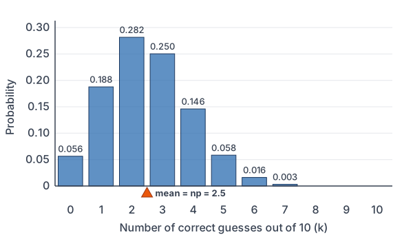
A student guesses on 10 multiple-choice questions, each with 4 choices. Let X be the number correct, so n = 10 and p = 0.25. Find P(X \ge 1) and P(X \le 2).
P(X = 0) = 0.75^{10} \approx 0.0563All 10 wrong. Each miss has probability 0.75.
P(X \ge 1) = 1 - P(X = 0)
Use the complement (see complement rule).
1 - 0.0563 = 0.9437
Subtract.
P(X = 1) = \binom{10}{1}(0.25)^1(0.75)^9Use the formula with k = 1.
\approx 10(0.25)(0.07508) \approx 0.1877
Evaluate, using 0.75⁹ ≈ 0.07508.
P(X = 2) = \binom{10}{2}(0.25)^2(0.75)^8Use the formula with k = 2.
\approx 45(0.0625)(0.10011) \approx 0.2816
Evaluate, using 0.75⁸ ≈ 0.10011.
P(X \le 2) = 0.0563 + 0.1877 + 0.2816
Add the probabilities for 0, 1 and 2.
= 0.5256
Add.
Answer: P(X \ge 1) \approx 0.9437 and P(X \le 2) \approx 0.5256. Check with binomcdf(10, 0.25, 2).
Example 4: Mean and standard deviation
For the guessing student in Example 3, find the mean and standard deviation of X.
\mu_X = np = 10(0.25)
Use the mean formula.
= 2.5
Multiply.
\sigma_X = \sqrt{np(1 - p)} = \sqrt{10(0.25)(0.75)}Use the standard deviation formula.
= \sqrt{1.875}Multiply.
\approx 1.37
Take the square root (see square roots).
Answer: on average a guesser gets 2.5 questions right, give or take about 1.37. The histogram shows the whole distribution.
Example 5: Defective phones (word problem)
A factory finds that 8% of its phones have a defect (example data). An inspector picks 20 phones at random from a large day’s production. Find the probability that no more than 1 is defective, and find the mean and standard deviation of the number defective.
n = 20, \ p = 0.08
20 is far less than 10% of a large day’s production, so the picks are close to independent.
P(X = 0) = 0.92^{20} \approx 0.1887All 20 are good.
P(X = 1) = \binom{20}{1}(0.08)(0.92)^{19}Use the formula with k = 1.
\approx 20(0.08)(0.2051)
Evaluate the power: 0.92¹⁹ ≈ 0.2051.
\approx 0.3282
Multiply.
P(X \le 1) = 0.1887 + 0.3282 = 0.5169
Add.
\mu_X = 20(0.08) = 1.6
Find the mean.
\sigma_X = \sqrt{20(0.08)(0.92)} = \sqrt{1.472}Multiply inside the root.
\approx 1.21
Take the square root.
Answer: P(X \le 1) \approx 0.5169, about a 52% chance. The inspector expects 1.6 defective phones, with a standard deviation of about 1.21.
Common mistakes
| Mistake | Example of the error | Fix |
|---|---|---|
| Leaving out n choose k | P(X = 3) = 0.7³ · 0.3² = 0.03087 | Multiply by the number of orders: 10 · 0.03087 = 0.3087. |
| Using binompdf for “at most” | binompdf(10, 0.25, 2) for P(X ≤ 2) | Use binomcdf for “at most”; binompdf gives exactly k. |
| Mixing up “at least” and “more than” | P(X ≥ 1) found as 1 − P(X ≤ 1) | At least 1 is 1 − P(X = 0). |
| Calling a “wait until” count binomial | Number of rolls until the first 6 | No fixed n: that is a geometric variable. |
| Forgetting the 10% condition | Sampling 5 of 20 students as if independent | Check that the sample is under 10% of the population. |
| Dropping the square root | σ = np(1 − p) = 1.875 | σ = √1.875 ≈ 1.37. |
Related methods
Where n choose k comes from
The coefficients \binom{n}{k} are the same numbers as in the binomial theorem and Pascal’s triangle. That is where the binomial distribution gets its name: the probabilities are the terms of (p + (1 - p))^n.
Using the mean and standard deviation
The mean and standard deviation formulas come from combining random variables. A binomial X is the sum of n independent trials. Each trial has mean p and variance p(1 - p), so the means and the variances add up n times.
Practice problems
- A coin is flipped 12 times, and X is the number of tails. Is X binomial? If so, give n and p.
- A die is rolled until a 6 appears, and X is the number of rolls. Is X binomial?
- X is binomial with n = 4 and p = 0.5. Find P(X = 2).
- X is binomial with n = 6 and p = 0.2. Find P(X = 0).
- Use Problem 4. Find P(X ≥ 1).
- A player makes 70% of her foul shots. Find the probability that she makes all 5 of 5 shots.
- X is binomial with n = 50 and p = 0.4. Find the mean and standard deviation.
- About 15% of people are left-handed. In a random group of 8 people, find the probability that exactly 2 are left-handed.
- X is binomial with n = 3 and p = 0.6. Find the whole probability distribution.
- A student guesses on 20 questions with 5 choices each. Find the mean and standard deviation of the number correct, and P(X = 0).
Show answers
1.
\text{2 outcomes, independent, } n = 12, \ p = 0.5All four BINS conditions hold.
Answer: yes, binomial with n = 12 and p = 0.5
2.
\text{no fixed } nYou stop when a 6 appears.
Answer: no; it is geometric
3.
\binom{4}{2} = 6Count the orders.
0.5^2 \cdot 0.5^2 = 0.0625
Probability of one order.
6(0.0625) = 0.375
Multiply.
Answer: 0.375
4.
\binom{6}{0} = 1Only one way to have no successes.
0.8^6 = 0.262144
All 6 are failures.
Answer: about 0.2621
5.
1 - 0.262144 = 0.737856
Use the complement.
Answer: about 0.7379
6.
0.7^5 = 0.16807
All 5 made; n choose k is 1.
Answer: about 0.1681
7.
\mu = 50(0.4) = 20
Mean = np.
\sigma = \sqrt{50(0.4)(0.6)} = \sqrt{12}Multiply inside the root.
\sqrt{12} \approx 3.46Take the square root.
Answer: mean 20, standard deviation about 3.46
8.
\binom{8}{2} = 28Count the orders.
0.15^2 = 0.0225
Two left-handed people.
0.85^6 \approx 0.37715
Six right-handed people.
28(0.0225)(0.37715) \approx 0.2376
Multiply.
Answer: about 0.2376
9.
P(X = 0) = 0.4^3 = 0.064
All failures.
P(X = 1) = 3(0.6)(0.4^2) = 0.288
Three orders.
P(X = 2) = 3(0.6^2)(0.4) = 0.432
Three orders.
P(X = 3) = 0.6^3 = 0.216
All successes.
0.064 + 0.288 + 0.432 + 0.216 = 1
Check that they add to 1.
Answer: 0.064, 0.288, 0.432 and 0.216 for X = 0, 1, 2, 3
10.
\mu = 20(0.2) = 4
Mean = np, with p = 1/5 = 0.2.
\sigma = \sqrt{20(0.2)(0.8)} = \sqrt{3.2}Multiply inside the root.
\sqrt{3.2} \approx 1.79Take the square root.
P(X = 0) = 0.8^{20} \approx 0.0115All 20 wrong.
Answer: mean 4, standard deviation about 1.79, P(X = 0) ≈ 0.0115
Binomial distribution FAQ
What are the 4 conditions for a binomial distribution?
Each trial has two outcomes, the trials are independent, the number of trials is fixed, and the probability of success is the same on every trial (BINS).
What is the difference between binompdf and binomcdf?
binompdf gives the probability of exactly k successes. binomcdf gives the probability of k or fewer successes.
How do you find the mean of a binomial distribution?
Multiply the number of trials by the probability of success: \mu = np. The standard deviation is \sqrt{np(1 - p)}.
How do you find “at least” binomial probabilities?
Use the complement. For example, P(X \ge 1) = 1 - P(X = 0), and P(X \ge 3) = 1 - P(X \le 2), which is 1 minus binomcdf(n, p, 2).
Summary
- A binomial random variable counts successes in n independent trials with the same success probability p (BINS).
- P(X = k) = \binom{n}{k} p^k (1 - p)^{n - k}.
- Mean np; standard deviation \sqrt{np(1 - p)}.
- Use binompdf for “exactly” and binomcdf for “at most”; use the complement for “at least.”
- When sampling without replacement, check that the sample is under 10% of the population.
Previous lesson: Combining Random Variables
Next lesson: Geometric Distribution
Back to the Statistics Index