
Expected Value
The expected value of a random variable X is its long-run average: the mean you would get if the random process were repeated many times. To find the expected value of a discrete random variable, multiply each value by its probability and add the products. It is written E(X) or \mu_X.
Before this lesson: Discrete Random Variables, Mean, Median, Mode and Range and Standard Deviation
What expected value means
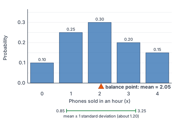
Picture a probability histogram as a seesaw. Each bar is a weight, and its height is its probability. The expected value is the balance point. Values with large probabilities pull the balance point toward them.
Expected value is an average over many repeats, not a prediction for one try. A store that sells 2.05 phones per hour on average never sells exactly 2.05 phones in one hour. Over hundreds of hours, though, the mean number sold will be close to 2.05.
The standard deviation of a random variable, \sigma_X, measures how far its values typically fall from the mean. It works like the standard deviation of a data set, but each squared deviation is weighted by its probability.
Expected value formula
For a discrete random variable X with values x and probabilities P(X = x):
\mu_X = E(X) = \sum x \cdot P(X = x)
The variance is the weighted average of the squared deviations from the mean. The standard deviation is its square root:
\sigma_X^2 = \sum (x - \mu_X)^2 \cdot P(X = x)
\sigma_X = \sqrt{\sigma_X^2}Calculator check: on a TI-84, put the values in L1 and the probabilities in L2. Then press STAT, CALC, 1:1-Var Stats, and enter L1 for the list and L2 for the frequency list. The calculator shows \mu_X as x̄ and \sigma_X as σx. In Desmos, type the values as a list x and the probabilities as a list p, then type total(x p) for the mean.
Expected value examples
Example 1: Number of heads in 3 flips
A coin is flipped 3 times. Let X be the number of heads. From discrete random variables, the distribution is P(0) = \tfrac{1}{8}, P(1) = \tfrac{3}{8}, P(2) = \tfrac{3}{8} and P(3) = \tfrac{1}{8}. Find E(X).
E(X) = 0 \cdot \dfrac{1}{8} + 1 \cdot \dfrac{3}{8} + 2 \cdot \dfrac{3}{8} + 3 \cdot \dfrac{1}{8}Multiply each value by its probability.
= \dfrac{0}{8} + \dfrac{3}{8} + \dfrac{6}{8} + \dfrac{3}{8}Multiply (see multiplying fractions).
= \dfrac{12}{8}Add the numerators (see adding fractions).
= 1.5
Divide.
Answer: E(X) = 1.5 heads. You can never get 1.5 heads in one set of flips, but over many sets of 3 flips the average is 1.5 heads.
Example 2: Mean number of phones sold
A phone store tracks X, the number of phones it sells in an hour (example data). Find the expected value.
| x | 0 | 1 | 2 | 3 | 4 |
|---|---|---|---|---|---|
| P(X = x) | 0.10 | 0.25 | 0.30 | 0.20 | 0.15 |
E(X) = 0(0.10) + 1(0.25) + 2(0.30) + 3(0.20) + 4(0.15)
Multiply each value by its probability.
= 0 + 0.25 + 0.60 + 0.60 + 0.60
Multiply (see operations with decimals).
= 2.05
Add.
Answer: \mu_X = 2.05 phones per hour. Over many hours, the store sells about 2.05 phones per hour on average.
Example 3: Standard deviation of phones sold
Find the variance and the standard deviation of X from Example 2. Use \mu_X = 2.05.
| x | x − μ | (x − μ)² | P(X = x) | (x − μ)² · P(X = x) |
|---|---|---|---|---|
| 0 | −2.05 | 4.2025 | 0.10 | 0.42025 |
| 1 | −1.05 | 1.1025 | 0.25 | 0.275625 |
| 2 | −0.05 | 0.0025 | 0.30 | 0.00075 |
| 3 | 0.95 | 0.9025 | 0.20 | 0.1805 |
| 4 | 1.95 | 3.8025 | 0.15 | 0.570375 |
0 - 2.05 = -2.05
Subtract the mean from each value; the table shows all five (see negative numbers).
(-2.05)^2 = 4.2025
Square each deviation (see exponents).
4.2025(0.10) = 0.42025
Multiply each square by its probability.
\sigma_X^2 = 0.42025 + 0.275625 + 0.00075 + 0.1805 + 0.570375
Add the last column.
\sigma_X^2 = 1.4475
This sum is the variance.
\sigma_X = \sqrt{1.4475}Take the square root (see square roots).
\sigma_X \approx 1.20
Round to the nearest hundredth.
Answer: the variance is 1.4475, and \sigma_X \approx 1.20 phones. In a typical hour, the number sold is about 1.2 phones away from the mean of 2.05.
Example 4: Is a carnival game worth playing? (word problem)
A carnival game costs $3 to play. You win $10 with probability 0.1 and $5 with probability 0.2. Otherwise you win nothing. Let X be your net gain: the prize minus the $3 cost. Find E(X).
10 - 3 = 7
Net gain for the $10 prize.
5 - 3 = 2
Net gain for the $5 prize.
0 - 3 = -3
Net gain when you win nothing.
1 - 0.1 - 0.2 = 0.7
Probability of winning nothing (see complement rule).
E(X) = 7(0.1) + 2(0.2) + (-3)(0.7)
Multiply each net gain by its probability.
= 0.7 + 0.4 - 2.1
Multiply (see multiplying integers).
= -1
Add.
Answer: E(X) = -1, so a player loses $1 per game on average. A game is fair when the expected net gain is 0. This one favors the carnival.
Example 5: Insurance company profit (word problem)
An insurance company sells a one-year phone policy for $120 (example data). It pays $900 if the phone is lost, with probability 0.03. It pays $200 for a screen repair, with probability 0.15. Let X be the company’s profit on one policy. Find the mean and the standard deviation of X.
120 - 900 = -780
Profit if the phone is lost.
120 - 200 = -80
Profit if the screen is repaired.
1 - 0.03 - 0.15 = 0.82
Probability of no claim, which gives a profit of $120.
\mu_X = -780(0.03) + (-80)(0.15) + 120(0.82)
Multiply each profit by its probability.
= -23.4 - 12 + 98.4
Multiply.
= 63
Add.
(-780 - 63)^2(0.03) = (-843)^2(0.03)
First squared deviation: subtract the mean.
(-843)^2(0.03) = 710649(0.03)
Square.
710649(0.03) = 21319.47
Multiply by the probability.
(-80 - 63)^2(0.15) = 20449(0.15)
Second value: subtract and square.
20449(0.15) = 3067.35
Multiply.
(120 - 63)^2(0.82) = 3249(0.82)
Third value: subtract and square.
3249(0.82) = 2664.18
Multiply.
\sigma_X^2 = 21319.47 + 3067.35 + 2664.18
Add the three products.
\sigma_X^2 = 27051
This is the variance.
\sigma_X = \sqrt{27051} \approx 164.47Take the square root and round.
Answer: the company earns $63 per policy on average, with a standard deviation of about $164.47. One policy is risky, but the company sells thousands, so its average profit per policy stays close to $63.
Common mistakes
| Mistake | Example of the error | Fix |
|---|---|---|
| Averaging the values without the probabilities | Mean phones = (0 + 1 + 2 + 3 + 4)/5 = 2 | Weight each value: 0(0.10) + 1(0.25) + … = 2.05. |
| Rounding the expected value to a possible value | “The store expects to sell 2 phones.” | Keep 2.05; it is a long-run average. |
| Forgetting to subtract the cost | Using $10 and $5 as the game’s gains | Net gain = prize − cost: 7, 2 and −3. |
| Taking the square root of each term | Adding square roots of the products | Add the products first to get the variance, then take one square root. |
| Squaring before subtracting the mean | Using x² · P(X = x) as the variance | Use (x − μ)² · P(X = x), or subtract μ² at the end (shortcut below). |
| Missing the “otherwise” outcome | Leaving out the 0.7 chance of winning nothing | Check that the probabilities add to 1. |
Related methods
Shortcut formula for the variance
You can also find the variance as the mean of the squares minus the square of the mean: \sigma_X^2 = E(X^2) - \mu_X^2. For the phones, E(X^2) = 0(0.10) + 1(0.25) + 4(0.30) + 9(0.20) + 16(0.15) = 5.65. Then 5.65 - 2.05^2 = 5.65 - 4.2025 = 1.4475, the same variance as Example 3.
Expected value from a data set
The mean of a data set from mean, median, mode and range is an expected value in disguise. Each data value’s relative frequency plays the part of its probability. The same idea gives the standard deviation of a data set. The next lesson, Combining Random Variables, finds the mean and standard deviation of sums and differences.
Practice problems
- X has values 1, 2 and 3 with probabilities 0.5, 0.3 and 0.2. Find E(X).
- A coin is flipped 2 times. Let X be the number of heads. Find E(X).
- Use the pets distribution from Discrete Random Variables: P(0) = 0.32, P(1) = 0.38, P(2) = 0.18, P(3) = 0.08, P(4) = 0.04. Find the mean number of pets.
- Find the variance and standard deviation of X in Problem 1.
- A fair die is rolled. Find the expected value of the number rolled.
- A game costs $1. You roll a die and win $4 if you roll a 6. Find the expected net gain.
- A game costs $2. You win a prize with probability 1/5. How big must the prize be for the game to be fair?
- Find the standard deviation of the number of heads in Problem 2.
- A $5 lottery ticket wins $1000 with probability 0.001 and $50 with probability 0.02. Find the expected net gain.
- Find the standard deviation of the net gain in Example 4’s carnival game.
Show answers
1.
1(0.5) + 2(0.3) + 3(0.2)
Multiply each value by its probability.
= 0.5 + 0.6 + 0.6
Multiply.
= 1.7
Add.
Answer: E(X) = 1.7
2.
0 \cdot \dfrac{1}{4} + 1 \cdot \dfrac{1}{2} + 2 \cdot \dfrac{1}{4}The distribution is 1/4, 1/2, 1/4.
= 0 + \dfrac{1}{2} + \dfrac{2}{4}Multiply.
= 1
Add.
Answer: E(X) = 1 head
3.
0(0.32) + 1(0.38) + 2(0.18) + 3(0.08) + 4(0.04)
Multiply each value by its probability.
= 0 + 0.38 + 0.36 + 0.24 + 0.16
Multiply.
= 1.14
Add.
Answer: 1.14 pets per household on average
4.
(1 - 1.7)^2 = 0.49
Square the first deviation from the mean.
0.49(0.5) = 0.245
Multiply by its probability.
(2 - 1.7)^2 = 0.09
Square the second deviation.
0.09(0.3) = 0.027
Multiply by its probability.
(3 - 1.7)^2 = 1.69
Square the third deviation.
1.69(0.2) = 0.338
Multiply by its probability.
\sigma_X^2 = 0.245 + 0.027 + 0.338 = 0.61
Add to get the variance.
\sigma_X = \sqrt{0.61} \approx 0.78Take the square root.
Answer: variance 0.61, standard deviation about 0.78
5.
\dfrac{1 + 2 + 3 + 4 + 5 + 6}{6}Each value has probability 1/6.
= \dfrac{21}{6}Add.
= 3.5
Divide.
Answer: 3.5
6.
4 - 1 = 3
Net gain on a 6.
3 \cdot \dfrac{1}{6} + (-1) \cdot \dfrac{5}{6}You lose $1 with probability 5/6.
= \dfrac{3}{6} - \dfrac{5}{6}Multiply.
= -\dfrac{2}{6} = -\dfrac{1}{3}Subtract and simplify.
Answer: about −$0.33 per game
7.
(W - 2) \cdot \dfrac{1}{5} + (-2) \cdot \dfrac{4}{5} = 0Let W be the prize. A fair game has E(X) = 0.
\dfrac{W}{5} - \dfrac{2}{5} - \dfrac{8}{5} = 0Distribute (see distributive property).
\dfrac{W}{5} - 2 = 0Combine the constants.
\dfrac{W}{5} = 2Add 2 to both sides.
W = 10
Multiply both sides by 5.
Answer: a $10 prize
8.
(0 - 1)^2 = 1
Square the first deviation from the mean, 1.
1 \cdot \dfrac{1}{4} = \dfrac{1}{4}Multiply by its probability.
(1 - 1)^2 = 0
The second deviation is 0, so its product is 0.
(2 - 1)^2 = 1
Square the third deviation.
1 \cdot \dfrac{1}{4} = \dfrac{1}{4}Multiply by its probability.
\sigma_X^2 = \dfrac{1}{4} + 0 + \dfrac{1}{4} = \dfrac{1}{2}Add.
\sigma_X = \sqrt{0.5} \approx 0.71Take the square root.
Answer: about 0.71 heads
9.
1000 - 5 = 995
Net gain for the $1000 prize.
50 - 5 = 45
Net gain for the $50 prize.
1 - 0.001 - 0.02 = 0.979
Probability of losing $5.
995(0.001) + 45(0.02) + (-5)(0.979)
Multiply each net gain by its probability.
= 0.995 + 0.9 - 4.895
Multiply.
= -3
Add.
Answer: −$3 per ticket on average
10.
(7 - (-1))^2 = 8^2 = 64
The mean is −1. Square the first deviation.
64(0.1) = 6.4
Multiply by its probability.
(2 - (-1))^2 = 3^2 = 9
Square the second deviation.
9(0.2) = 1.8
Multiply by its probability.
(-3 - (-1))^2 = (-2)^2 = 4
Square the third deviation.
4(0.7) = 2.8
Multiply by its probability.
\sigma_X^2 = 6.4 + 1.8 + 2.8 = 11
Add.
\sigma_X = \sqrt{11} \approx 3.32Take the square root.
Answer: about $3.32
Expected value FAQ
What is the expected value in statistics?
It is the mean of a random variable: the long-run average outcome if the process is repeated many times. For a discrete random variable, it is the sum of each value times its probability.
Can the expected value be a number X can never equal?
Yes. The expected number of heads in 3 flips is 1.5, even though no single set of flips gives 1.5 heads. It describes the average over many repeats.
What does a negative expected value mean?
If X is a net gain, a negative expected value means you lose money on average over many plays. Casino games and lotteries have negative expected values for players.
How do you find the standard deviation of a random variable?
Subtract the mean from each value, square the result and multiply by its probability. Add these products to get the variance, then take the square root.
Summary
- The expected value is the long-run average of a random variable: \mu_X = \sum x \cdot P(X = x).
- It is the balance point of the probability histogram and need not be a possible value.
- The variance is \sum (x - \mu_X)^2 \cdot P(X = x), and the standard deviation is its square root.
- For games and insurance, define X as the net gain, then find its expected value.
- A game is fair when the expected net gain is 0.
Previous lesson: Discrete Random Variables
Next lesson: Combining Random Variables
Back to the Statistics Index