
Normal Distribution
A normal distribution is a symmetric, bell-shaped distribution of a continuous variable. Two numbers set it: the mean μ, which is the center of the curve, and the standard deviation σ, which sets how spread out it is. Many real measurements, like heights and birth weights, are close to normal.
Before this lesson: Density Curves, Standard Deviation and Percentiles and Z-Scores
What a normal distribution looks like
Picture the weights of thousands of newborn babies. Most are near the average. Fewer are much lighter or much heavier. A histogram of the weights rises to one peak in the middle and falls off evenly on both sides.
A smooth curve drawn over that histogram is a normal curve, also called a bell curve. It is a density curve, so the total area under it is 1. The area over an interval is the probability of a value in that interval.
Normal distribution properties
- It has one peak, at the mean μ.
- It is symmetric about the mean, so the mean and the median are equal (see describing a distribution).
- Half of the area is on each side of the mean.
- It never touches the horizontal axis. The tails get closer and closer to it but go on forever.
- The curve changes from bending down to bending up at μ − σ and μ + σ. These two points are the inflection points.
We write a normal distribution with mean μ and standard deviation σ as N(\mu, \sigma). For example, N(3400, 500) has mean 3,400 and standard deviation 500.
Normal distribution formula
The height of the normal curve at each value x is given by this formula:
f(x) = \dfrac{1}{\sigma\sqrt{2\pi}}\, e^{-\frac{(x - \mu)^2}{2\sigma^2}}You won’t use this formula to find areas by hand. Tables and calculators do that. But it shows two useful facts. The highest point is at x = μ, where the height is \dfrac{1}{\sigma\sqrt{2\pi}}. And a bigger σ gives a lower peak, because the curve gets wider and the area must stay 1.
How μ and σ change the curve
- Changing μ slides the whole curve left or right. The shape stays the same.
- Changing σ stretches or squeezes the curve. A small σ gives a tall, narrow curve. A large σ gives a short, wide one.
Normal distribution examples
Example 1: Find μ and σ from a graph
A normal curve has its peak at x = 70. Its inflection points are at x = 64 and x = 76. Find the mean and the standard deviation.
\mu = \dfrac{64 + 76}{2}The curve is symmetric, so the mean is halfway between the inflection points.
= \dfrac{140}{2}Add.
= 70
Divide. This matches the peak.
\sigma = 76 - 70
An inflection point is one standard deviation from the mean.
= 6
Subtract.
Answer: μ = 70 and σ = 6, so the distribution is N(70, 6).
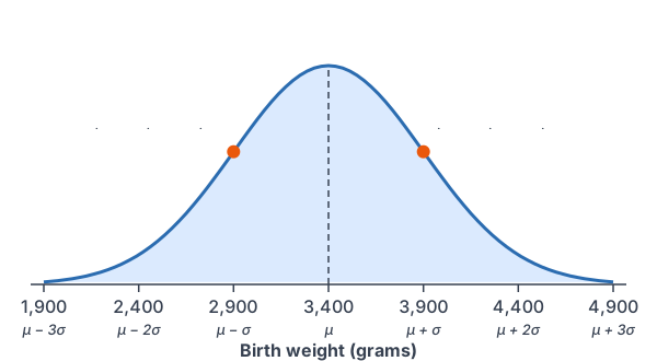
Example 2: Label a normal curve (birth weights)
Birth weights of full-term babies are approximately normal with mean 3,400 grams and standard deviation 500 grams. Find the values 1, 2 and 3 standard deviations from the mean.
2\sigma = 2(500) = 1000
Find two standard deviations.
3\sigma = 3(500) = 1500
Find three standard deviations.
3400 \pm 500 = 2900 \text{ and } 3900Subtract and add one standard deviation.
3400 \pm 1000 = 2400 \text{ and } 4400Subtract and add two standard deviations.
3400 \pm 1500 = 1900 \text{ and } 4900Subtract and add three standard deviations.
Answer: from left to right, 1,900, 2,400, 2,900, 3,400, 3,900, 4,400 and 4,900 grams. These are the marks on the graph above.
Example 3: Use symmetry to find areas
Use the birth weights from Example 2. The probability that a baby weighs less than 2,400 grams is about 0.0228. Find P(X \gt 3400), P(X \gt 4400) and P(2400 \lt X \lt 4400).
P(X \gt 3400) = 0.5
Half of the area is above the mean.
4400 - 3400 = 1000
4,400 is 1,000 above the mean.
3400 - 2400 = 1000
2,400 is 1,000 below the mean, the same distance.
P(X \gt 4400) = P(X \lt 2400)
By symmetry, the two tails have equal areas.
\approx 0.0228
Use the given value.
P(2400 \lt X \lt 4400) \approx 1 - 2(0.0228)
Take both tails away from the total area of 1 (see complement rule).
= 1 - 0.0456
Multiply.
= 0.9544
Subtract.
Answer: P(X \gt 3400) = 0.5, P(X \gt 4400) \approx 0.0228 and P(2400 \lt X \lt 4400) \approx 0.9544. About 95% of babies weigh between 2,400 and 4,400 grams.
Example 4: Compare two normal curves
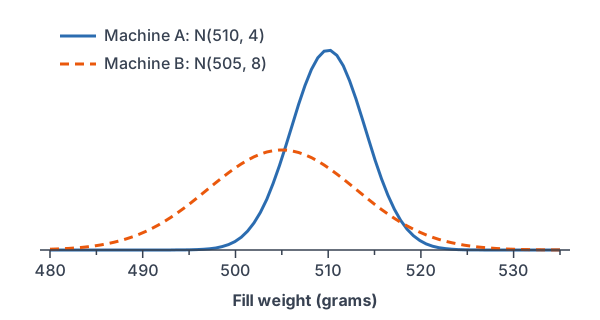
Two machines fill cereal boxes. Machine A’s fill weights are N(510, 4) grams. Machine B’s are N(505, 8) grams. Which curve is centered farther right? Which is taller? Find each peak height.
510 \gt 505
Compare the means: A is centered farther right.
\dfrac{1}{4\sqrt{2\pi}} \approx \dfrac{1}{10.027}Peak height of A: put σ = 4 in the peak formula, and use 4√(2π) ≈ 10.027 (see square roots).
\approx 0.0997
Divide.
\dfrac{1}{8\sqrt{2\pi}} \approx \dfrac{1}{20.053}Peak height of B, with σ = 8.
\approx 0.0499
Divide.
\dfrac{0.0997}{0.0499} \approx 2Compare the heights.
Answer: A is centered farther right, at 510 g. A’s curve is about twice as tall, since its σ is half as big. B’s curve is lower and wider, so its fills vary more.
Example 5: Which value is more unusual? (word problem)
Newborn lengths are approximately normal with mean 50 cm and standard deviation 2 cm. One baby is 54 cm long and weighs 4,650 grams. Use the weights from Example 2. Is this baby more unusual in length or in weight?
z = \dfrac{x - \mu}{\sigma}A z-score counts standard deviations from the mean (see z-scores).
z_{\text{length}} = \dfrac{54 - 50}{2}Substitute the length values.
= \dfrac{4}{2}Subtract.
= 2
Divide.
z_{\text{weight}} = \dfrac{4650 - 3400}{500}Substitute the weight values.
= \dfrac{1250}{500}Subtract.
= 2.5
Divide.
2.5 \gt 2
Compare the z-scores.
Answer: the weight is 2.5 standard deviations above the mean, and the length is 2 above. The weight is more unusual.
Common mistakes
| Mistake | Example of the error | Fix |
|---|---|---|
| Mixing up the order in N(μ, σ) | Reading N(70, 6) as a mean of 6 | The first number is the mean. The second is the standard deviation. |
| Using the variance as σ | Treating a variance of 36 as σ = 36 | Take the square root: σ = 6. |
| Putting the inflection points in the wrong place | Inflection points of N(70, 6) at 58 and 82 | They are one σ from the mean: 64 and 76. |
| Thinking a larger σ means a taller curve | Saying N(505, 8) is taller than N(510, 4) | A larger σ makes the curve lower and wider. |
| Thinking the tails stop | P(X > 4,900) = 0 for birth weights | The curve never touches the axis. The area is small, but not 0. |
| Calling any mound-shaped data normal | Calling a skewed histogram normal | A normal curve is symmetric with one peak. |
Related methods
The empirical rule
In Example 3, about 95% of the area was within 2 standard deviations of the mean. That is true for every normal curve. The next lesson, Empirical Rule, gives the shares for 1, 2 and 3 standard deviations.
Z-scores and other distributions
A z-score turns any normal variable into N(0, 1), the standard normal distribution. Then one table works for every normal curve. A later lesson uses z-scores to find areas. Some other distributions, like the binomial distribution with many trials, also have a bell shape.
Practice problems
- A normal curve peaks at 120, and its inflection points are at 105 and 135. Find μ and σ.
- X is N(80, 5). Find the values 1, 2 and 3 standard deviations below and above the mean.
- X is N(80, 5). Find P(X \gt 80).
- X is N(80, 5), and P(X \lt 72) \approx 0.0548. Find P(X \gt 88).
- Use Problem 4. Find P(72 \lt X \lt 88).
- Which curve has the taller peak, N(50, 2) or N(40, 10)? How many times as tall is it?
- Find the peak height of N(0, 1) to four decimal places.
- Test scores are N(72, 8). How many standard deviations above the mean is a score of 88?
- Maya scored 84 on a quiz where scores were N(75, 6) and 90 on a quiz where scores were N(82, 4). On which quiz did she do better compared with her class?
- A normal curve has inflection points at 3.2 and 4.8. Find μ and σ.
Show answers
1.
\mu = \dfrac{105 + 135}{2}The mean is halfway between the inflection points.
= \dfrac{240}{2}Add.
= 120
Divide. It matches the peak.
\sigma = 135 - 120 = 15
Distance from the mean to an inflection point.
Answer: μ = 120 and σ = 15
2.
2\sigma = 2(5) = 10
Two standard deviations.
3\sigma = 3(5) = 15
Three standard deviations.
80 \pm 5 = 75 \text{ and } 85One standard deviation below and above.
80 \pm 10 = 70 \text{ and } 90Two standard deviations below and above.
80 \pm 15 = 65 \text{ and } 95Three standard deviations below and above.
Answer: 65, 70, 75, 85, 90 and 95
3.
P(X \gt 80) = 0.5
Half of the area is above the mean.
Answer: 0.5
4.
88 - 80 = 8
88 is 8 above the mean.
80 - 72 = 8
72 is 8 below the mean.
P(X \gt 88) = P(X \lt 72)
Equal distances give equal tail areas.
\approx 0.0548
Use the given value.
Answer: about 0.0548
5.
P(72 \lt X \lt 88) \approx 1 - 2(0.0548)
Take both tails away from the total area.
= 1 - 0.1096
Multiply.
= 0.8904
Subtract.
Answer: about 0.8904
6.
\dfrac{1}{2\sqrt{2\pi}} \approx 0.1995Peak height of N(50, 2).
\dfrac{1}{10\sqrt{2\pi}} \approx 0.0399Peak height of N(40, 10).
\dfrac{0.1995}{0.0399} = 5Divide the heights.
Answer: N(50, 2) has the taller peak, 5 times as tall
7.
\sqrt{2\pi} \approx 2.5066Find the square root of 2π.
\dfrac{1}{2.5066} \approx 0.3989Divide.
Answer: about 0.3989
8.
z = \dfrac{88 - 72}{8}Substitute into the z-score formula.
= \dfrac{16}{8}Subtract.
= 2
Divide.
Answer: 2 standard deviations above the mean
9.
z_1 = \dfrac{84 - 75}{6}z-score on the first quiz.
= \dfrac{9}{6}Subtract.
= 1.5
Divide.
z_2 = \dfrac{90 - 82}{4}z-score on the second quiz.
= \dfrac{8}{4}Subtract.
= 2
Divide.
2 \gt 1.5
Compare the z-scores.
Answer: the second quiz
10.
\mu = \dfrac{3.2 + 4.8}{2}The mean is halfway between the inflection points.
= \dfrac{8}{2}Add.
= 4
Divide.
\sigma = 4.8 - 4 = 0.8
Distance from the mean to an inflection point.
Answer: μ = 4 and σ = 0.8
Normal distribution FAQ
What is a normal distribution in statistics?
It is a symmetric, bell-shaped distribution for a continuous variable. Its center is the mean μ, and its spread is the standard deviation σ.
What do μ and σ tell you about a normal curve?
μ is where the peak is. σ is the distance from the mean to each inflection point, so a bigger σ means a wider, lower curve.
Why is it called a bell curve?
Its graph has one rounded peak in the middle and tails that slope down evenly on both sides, like the outline of a bell.
Is all bell-shaped data normal?
No. Data can be mound-shaped but skewed, or have heavier tails than a normal curve. A later lesson, Normal Probability Plots, shows how to check.
Summary
- A normal distribution N(\mu, \sigma) is symmetric and bell-shaped, with one peak at the mean.
- The mean and median are equal, and half of the area is on each side.
- The inflection points are at μ − σ and μ + σ.
- A larger σ gives a lower, wider curve. Changing μ slides the curve.
- The total area is 1, and the tails never touch the axis.
Previous lesson: Density Curves
Next lesson: Empirical Rule
Back to the Statistics Index