
Normal Approximation to the Binomial
The normal approximation to the binomial uses a normal curve to estimate binomial probabilities when the number of trials is large. If np ≥ 10 and n(1 − p) ≥ 10, the binomial count X is close to normal, with mean np and standard deviation \sqrt{np(1 - p)}.
Before this lesson: Binomial Distribution, Normal Distribution and Normal Probability Calculations
Why a binomial can look normal
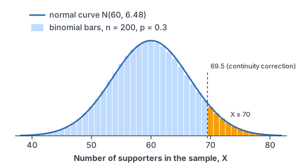
A binomial count X is the number of successes in n independent trials, each with success probability p. With only a few trials, its histogram is often skewed. With many trials, the bars form a smooth, nearly symmetric mound.
That mound is close to a normal curve with the same mean and standard deviation. So you can estimate a binomial probability with a z-score and the z-table, without adding up dozens of binomial terms.
Conditions and formulas
Use the normal approximation only when the large counts condition holds: np ≥ 10 and n(1 − p) ≥ 10. That means at least 10 expected successes and at least 10 expected failures. (Some books use 5 instead of 10.)
\mu = np \qquad \sigma = \sqrt{np(1 - p)}These are the same mean and standard deviation as the binomial, from expected value rules. Then X is approximately N\left(np, \sqrt{np(1 - p)}\right).
The continuity correction
A binomial count takes only whole numbers, but the normal curve is continuous. The bar for a whole number k covers k − 0.5 to k + 0.5. Moving each boundary by 0.5 to match the bars is called the continuity correction.
| Binomial question | Normal area to use |
|---|---|
| P(X ≥ 70) | P(X > 69.5) |
| P(X > 70) | P(X > 70.5) |
| P(X ≤ 90) | P(X < 90.5) |
| P(X < 90) | P(X < 89.5) |
| P(X = 50) | P(49.5 < X < 50.5) |
AP Statistics usually skips the continuity correction, and many college courses use it. It brings the estimate closer to the exact answer. If your class skips it, use the boundary itself, as in Example 3.
Calculator: for the exact binomial answer, use binomcdf(n, p, k) on a TI-84, or binomialdist(n, p).cdf(k) in Desmos. For the normal estimate, use normalcdf with μ = np and σ = √(np(1 − p)).
Normal approximation examples
Example 1: Check the conditions
Can you use the normal approximation for (a) n = 200 and p = 0.3? (b) n = 40 and p = 0.1?
200(0.3) = 60
(a) Expected successes, np.
200(0.7) = 140
Expected failures, n(1 − p).
60 \ge 10 \text{ and } 140 \ge 10Both are at least 10, so the approximation is OK.
40(0.1) = 4
(b) Expected successes, np.
4 \lt 10
Too few expected successes.
Answer: (a) yes; (b) no. With only 4 expected successes, that binomial is skewed right, so a normal curve fits poorly.
Example 2: Find the mean and standard deviation
Suppose 30% of a city’s voters support a new library. A poll takes a random sample of 200 voters. X is the number of supporters in the sample. Find the mean and standard deviation of X.
\mu = 200(0.3) = 60
Multiply n by p.
60(0.7) = 42
Multiply np by 1 − p.
\sigma = \sqrt{42} \approx 6.48Take the square root (see square roots).
Answer: μ = 60 and σ ≈ 6.48, so X is approximately N(60, 6.48). Example 1 showed the conditions hold.
Example 3: Estimate a probability without the correction
Use the poll from Example 2. Estimate the probability that 70 or more voters in the sample support the library. Don’t use the continuity correction.
z = \dfrac{70 - 60}{6.48}Change 70 to a z-score.
= \dfrac{10}{6.48}Subtract.
\approx 1.54
Divide.
P(Z \lt 1.54) = 0.9382
Read the z-table.
1 - 0.9382 = 0.0618
70 or more is the right area (see complement rule).
Answer: about 0.0618. The exact binomial answer, 1 − binomcdf(200, 0.3, 69), is about 0.0728.
Example 4: Use the continuity correction
Repeat Example 3 with the continuity correction.
P(X \ge 70) \approx P(X \gt 69.5)
The bar for 70 starts at 69.5.
z = \dfrac{69.5 - 60}{6.48}Change 69.5 to a z-score.
= \dfrac{9.5}{6.48}Subtract.
\approx 1.47
Divide.
P(Z \lt 1.47) = 0.9292
Read the z-table.
1 - 0.9292 = 0.0708
Take the right area.
Answer: about 0.0708. That is much closer to the exact 0.0728 than the estimate without the correction.
Example 5: Overbooking a flight (word problem)
An airline sells 190 tickets for a flight with 180 seats. Each ticket holder shows up with probability 0.94, independently of the others. Estimate the probability that more than 180 people show up.
190(0.94) = 178.6
Expected arrivals, np.
190(0.06) = 11.4
Expected no-shows, n(1 − p). Both are at least 10.
178.6(0.06) = 10.716
Find np(1 − p).
\sigma = \sqrt{10.716} \approx 3.27Take the square root.
P(X \gt 180) \approx P(X \gt 180.5)
More than 180 means 181 or more, and the bar for 181 starts at 180.5.
z = \dfrac{180.5 - 178.6}{3.27}Change 180.5 to a z-score.
= \dfrac{1.9}{3.27}Subtract.
\approx 0.58
Divide.
1 - 0.7190 = 0.2810
P(Z \lt 0.58) = 0.7190, so take the right area.
Answer: about 0.28, so more than 1 flight in 4 like this would be overbooked. The exact answer, 1 − binomcdf(190, 0.94, 180), is about 0.29.
Common mistakes
| Mistake | Example of the error | Fix |
|---|---|---|
| Skipping the condition check | Using a normal curve for n = 40, p = 0.1 | Check np ≥ 10 and n(1 − p) ≥ 10 first. |
| Using the variance as σ | Using σ = 42 for the poll | Take the square root: σ = √42 ≈ 6.48. |
| Correcting in the wrong direction | P(X ≥ 70) ≈ P(X > 70.5) | At least 70 includes the bar for 70, so start at 69.5. |
| Treating “more than” like “at least” | P(X > 180) ≈ P(X > 179.5) | More than 180 starts at 181, so use 180.5. |
| Saying P(X = k) is 0 | P(X = 50) = 0 because the curve is continuous | Use the bar: P(49.5 < X < 50.5). |
| Mixing a proportion with a count | z = (70 − 0.3)/6.48 | Use counts: the mean is np = 60. |
Related methods
Exact answers with technology
A calculator finds exact binomial probabilities with binomcdf, so you can check any estimate. The normal approximation still matters because it explains why counts and proportions from large samples are close to normal.
Sample proportions
Divide the count by n to get the sample proportion. Its mean is p, and its standard deviation is \sqrt{\dfrac{p(1 - p)}{n}}. A later lesson, Sampling Distribution of a Sample Proportion, builds on this.
Practice problems
- For n = 50 and p = 0.4, can you use the normal approximation?
- For n = 60 and p = 0.05, can you use the normal approximation?
- For n = 400 and p = 0.25, find the mean and standard deviation of X.
- Use Problem 3. Estimate P(X ≤ 90) with the continuity correction.
- A fair coin is flipped 100 times. Estimate the probability of at least 60 heads, with the continuity correction.
- Write the continuity-corrected normal area for (a) P(X ≥ 45) and (b) P(X < 30).
- A fair coin is flipped 100 times. Estimate the probability of exactly 50 heads.
- In a large town, 62% of adults own a pet. In a random sample of 1,000 adults, estimate P(X ≥ 650), with the continuity correction.
- Why does the approximation need np ≥ 10 and n(1 − p) ≥ 10?
- A gardener plants 300 seeds, and each grows with probability 0.85. Estimate the probability that fewer than 245 grow, with the continuity correction.
Show answers
1.
50(0.4) = 20
Expected successes.
50(0.6) = 30
Expected failures. Both are at least 10.
Answer: yes
2.
60(0.05) = 3
Expected successes.
3 \lt 10
The condition fails.
Answer: no
3.
\mu = 400(0.25) = 100
Multiply n by p.
100(0.75) = 75
Multiply np by 1 − p.
\sigma = \sqrt{75} \approx 8.66Take the square root.
Answer: μ = 100 and σ ≈ 8.66
4.
P(X \le 90) \approx P(X \lt 90.5)
The bar for 90 ends at 90.5.
z = \dfrac{90.5 - 100}{8.66} = \dfrac{-9.5}{8.66}Change 90.5 to a z-score: subtract.
\approx -1.10
Divide.
P(Z \lt -1.10) = 0.1357
Read the z-table.
Answer: about 0.1357 (exact: about 0.1358)
5.
\mu = 100(0.5) = 50
Mean.
100(0.5)(0.5) = 25
Find np(1 − p).
\sigma = \sqrt{25} = 5Take the square root.
P(X \ge 60) \approx P(X \gt 59.5)
Continuity correction.
z = \dfrac{59.5 - 50}{5} = \dfrac{9.5}{5}Subtract.
= 1.9
Divide.
1 - 0.9713 = 0.0287
P(Z \lt 1.90) = 0.9713, so take the right area.
Answer: about 0.0287 (exact: about 0.0284)
6.
P(X \ge 45) \approx P(X \gt 44.5)
At least 45 includes the bar for 45, which starts at 44.5.
P(X \lt 30) \approx P(X \lt 29.5)
Less than 30 stops at 29, whose bar ends at 29.5.
Answer: (a) P(X > 44.5); (b) P(X < 29.5)
7.
P(X = 50) \approx P(49.5 \lt X \lt 50.5)
Use the bar for 50.
z = \dfrac{49.5 - 50}{5} = \dfrac{-0.5}{5}Lower z: subtract.
= -0.1
Divide.
z = \dfrac{50.5 - 50}{5} = \dfrac{0.5}{5}Upper z: subtract.
= 0.1
Divide.
0.5398 - 0.4602 = 0.0796
Subtract the left areas.
Answer: about 0.0796 (exact: about 0.0796)
8.
\mu = 1000(0.62) = 620
Mean.
620(0.38) = 235.6
Multiply np by 1 − p.
\sigma = \sqrt{235.6} \approx 15.35Take the square root.
z = \dfrac{649.5 - 620}{15.35} = \dfrac{29.5}{15.35}Use 649.5, then subtract.
\approx 1.92
Divide.
1 - 0.9726 = 0.0274
P(Z \lt 1.92) = 0.9726, so take the right area.
Answer: about 0.0274 (exact: about 0.0268)
9.
With fewer than 10 expected successes or failures, the binomial is skewed, so a symmetric normal curve fits it poorly.
Answer: they make sure the binomial is close enough to symmetric for a normal curve
10.
\mu = 300(0.85) = 255
Mean. The expected failures, 45, are at least 10.
255(0.15) = 38.25
Multiply np by 1 − p.
\sigma = \sqrt{38.25} \approx 6.18Take the square root.
P(X \lt 245) \approx P(X \lt 244.5)
Fewer than 245 means 244 or fewer.
z = \dfrac{244.5 - 255}{6.18} = \dfrac{-10.5}{6.18}Subtract.
\approx -1.70
Divide.
P(Z \lt -1.70) = 0.0446
Read the z-table.
Answer: about 0.0446 (exact: about 0.0478)
Normal approximation FAQ
When can you use the normal approximation to the binomial?
When np ≥ 10 and n(1 − p) ≥ 10. Then the binomial distribution is close enough to symmetric for a normal curve.
What is the mean and standard deviation for the normal approximation?
Use the binomial’s own values: μ = np and σ = √(np(1 − p)).
What is the continuity correction?
It moves each boundary by 0.5 so the normal curve covers whole bars of the binomial histogram. For example, P(X ≥ 70) becomes P(X > 69.5).
Do you need the continuity correction on the AP Statistics exam?
AP Statistics usually does not use it. Many college courses do, and it gives an estimate closer to the exact answer.
Summary
- A binomial count X is close to normal when np ≥ 10 and n(1 − p) ≥ 10.
- Use μ = np and σ = √(np(1 − p)).
- The continuity correction moves each boundary by 0.5 to match the bars.
- At least k starts at k − 0.5. More than k starts at k + 0.5.
- Check estimates with binomcdf when you have a calculator.
Previous lesson: Normal Probability Plots
Next lesson: Sampling Distributions
Back to the Statistics Index