Sampling Distribution of a Difference

A sampling distribution for a difference describes how p̂₁ − p̂₂ or x̄₁ − x̄₂ varies when you take two independent random samples. Its mean is the difference in the population values. Its standard deviation comes from adding the two variances, then taking the square root. With large enough samples, its shape is approximately normal.

Before this lesson: Sampling Distribution of a Sample Proportion, Sampling Distribution of a Sample Mean and Combining Random Variables

Why study differences?

Many questions compare two groups. Do more students ride the bus at School A than at School B? Do first-year students sleep more than seniors? To answer, you take a sample from each group and compare the results.

Even if the two groups were exactly alike, the two samples would not match. So you need to know how much the difference between two sample results varies by chance. That is what this sampling distribution tells you.

The key fact comes from combining random variables: when you subtract two independent random variables, their variances add. A difference varies more than either sample result alone.

Formulas for differences

Difference in sample proportions

\mu_{\hat{p}_1 - \hat{p}_2} = p_1 - p_2 \qquad \sigma_{\hat{p}_1 - \hat{p}_2} = \sqrt{\dfrac{p_1(1 - p_1)}{n_1} + \dfrac{p_2(1 - p_2)}{n_2}}

The shape is approximately normal when all four counts are at least 10: $n_1p_1$ , $n_1(1 - p_1)$ , $n_2p_2$ and $n_2(1 - p_2)$ .

Difference in sample means

\mu_{\bar{x}_1 - \bar{x}_2} = \mu_1 - \mu_2 \qquad \sigma_{\bar{x}_1 - \bar{x}_2} = \sqrt{\dfrac{\sigma_1^2}{n_1} + \dfrac{\sigma_2^2}{n_2}}

The shape is normal when both populations are normal. It is approximately normal when both samples have n ≥ 30.

Conditions for both

Random and independent: two independent random samples, or two groups formed by random assignment in an experiment.
10% condition: each sample is less than 10% of its population.
Normal shape: Large Counts for proportions, or Normal/Large Sample for means.

Calculator: find the standard deviation first, then use normalcdf(lower, upper, mean, SD) on a TI-84 or normaldist(mean, SD).cdf(a, b) in Desmos.

Sampling distributions for differences examples

Example 1: Describe the distribution of p̂₁ − p̂₂

At School A, 60% of students ride the bus. At School B, 45% do. Random samples of 100 students from A and 120 from B are taken. Describe the sampling distribution of p̂₁ − p̂₂.

\mu = 0.60 - 0.45 = 0.15

The mean is the difference in population proportions.

0.60(0.40) = 0.24

Variance of p̂₁: multiply p₁ by 1 − p₁.

\dfrac{0.24}{100} = 0.0024

Divide by n₁.

0.45(0.55) = 0.2475

Variance of p̂₂: multiply p₂ by 1 − p₂.

\dfrac{0.2475}{120} = 0.0020625

Divide by n₂.

0.0024 + 0.0020625 = 0.0044625

Add the variances (see combining random variables).

\sigma = \sqrt{0.0044625} \approx 0.0668

Take the square root (see square roots).

Large Counts: 100(0.60) = 60, 100(0.40) = 40, 120(0.45) = 54 and 120(0.55) = 66 are all at least 10.

Answer: approximately normal, with mean 0.15 and standard deviation about 0.0668.

Example 2: Probability for a difference in proportions

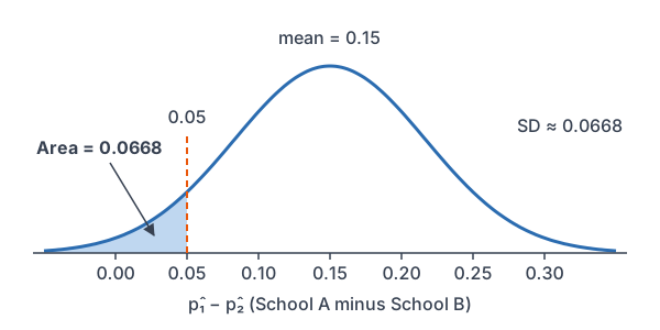
Use Example 1. What is the probability that School A’s sample proportion is less than 0.05 above School B’s?

z = \dfrac{0.05 - 0.15}{0.0668} = \dfrac{-0.10}{0.0668}

Change 0.05 to a z-score: subtract.

\approx -1.50

Divide.

P(Z \lt -1.50) = 0.0668

Read the z-table (see standard normal distribution).

Answer: about 0.0668. The real gap is 15 points, so seeing a gap under 5 points in the samples would be unusual.

Example 3: Describe the distribution of x̄₁ − x̄₂

At a large university, first-year students sleep a mean of 7.2 hours a night with standard deviation 1.2 hours. Seniors sleep a mean of 6.9 hours with standard deviation 1.4 hours. Random samples of 36 first-year students and 49 seniors are taken. Describe the sampling distribution of x̄₁ − x̄₂.

\mu = 7.2 - 6.9 = 0.3

The mean is the difference in population means.

1.2^2 = 1.44

Variance of x̄₁: square σ₁.

\dfrac{1.44}{36} = 0.04

Divide by n₁.

1.4^2 = 1.96

Variance of x̄₂: square σ₂.

\dfrac{1.96}{49} = 0.04

Divide by n₂.

0.04 + 0.04 = 0.08

Add the variances.

\sigma = \sqrt{0.08} \approx 0.2828

Take the square root.

36 \ge 30 \text{ and } 49 \ge 30

Both samples are large, so the shape is approximately normal.

Answer: approximately normal, with mean 0.3 hours and standard deviation about 0.2828 hours.

Example 4: Chance the order flips

Use Example 3. What is the probability that the seniors’ sample mean is higher than the first-year students’ sample mean?

\bar{x}_1 - \bar{x}_2 \lt 0

Seniors higher means the difference is negative.

z = \dfrac{0 - 0.3}{0.2828} = \dfrac{-0.3}{0.2828}

Change 0 to a z-score: subtract.

\approx -1.06

Divide.

P(Z \lt -1.06) = 0.1446

Read the z-table.

Answer: about 0.1446. Even though first-year students sleep more on average, about 1 pair of samples in 7 would show the opposite.

Example 5: Comparing two factories (word problem)

Factory 1 makes phone screens with a 4% defect rate. Factory 2 has a 2% rate. An inspector takes random samples of 500 screens from Factory 1 and 600 from Factory 2. What is the probability that Factory 1’s sample defect rate is more than 4 percentage points higher than Factory 2’s?

Large Counts: 500(0.04) = 20, 500(0.96) = 480, 600(0.02) = 12 and 600(0.98) = 588 are all at least 10.

\mu = 0.04 - 0.02 = 0.02

Find the mean difference.

0.04(0.96) = 0.0384

Factory 1: multiply p₁ by 1 − p₁.

\dfrac{0.0384}{500} = 0.0000768

Divide by n₁.

0.02(0.98) = 0.0196

Factory 2: multiply p₂ by 1 − p₂.

\dfrac{0.0196}{600} \approx 0.0000327

Divide by n₂.

0.0000768 + 0.0000327 = 0.0001095

Add the variances.

\sigma = \sqrt{0.0001095} \approx 0.01046

Take the square root.

z = \dfrac{0.04 - 0.02}{0.01046} = \dfrac{0.02}{0.01046}

Change 0.04 to a z-score: subtract.

\approx 1.91

Divide.

1 - 0.9719 = 0.0281

$P(Z \lt 1.91) = 0.9719$ , so take the right area (see complement rule).

Answer: about 0.0281. A gap that large would be rare if the true rates are 4% and 2%.

Common mistakes

Mistake	Example of the error	Fix
Subtracting the variances	0.0024 − 0.0020625 for p̂₁ − p̂₂	Variances always add, even for a difference.
Adding standard deviations	$\sqrt{0.0024} + \sqrt{0.0020625}$	Add the variances first, then take one square root.
Using one sample size for both groups	Dividing both variances by 100	Divide each variance by its own n.
Checking Large Counts for one group only	Checking 60 and 40 but not School B	Check all four counts.
Mixing up the order	Mean 0.45 − 0.60 when the question is about p̂₁ − p̂₂	Keep the same order (group 1 minus group 2) all the way through.

Related methods

Where this leads

Confidence intervals and significance tests for two proportions and two means start from these sampling distributions. In those lessons, the unknown p₁, p₂, σ₁ and σ₂ are replaced by their sample values.

Single-sample versions

Each piece of the formula is the variance from a one-sample sampling distribution. If you know the central limit theorem and the one-sample formulas, the two-sample versions follow from adding variances.

Practice problems

For two groups, p₁ = 0.5 with n₁ = 200, and p₂ = 0.4 with n₂ = 150. Find the mean and standard deviation of p̂₁ − p̂₂.
Use Problem 1. Check the Large Counts condition.
Use Problem 1. Find $P(\hat{p}_1 - \hat{p}_2 \gt 0.2)$ .
Two populations have μ₁ = 50 and μ₂ = 46. Find the mean of x̄₁ − x̄₂.
Use Problem 4 with σ₁ = 6, n₁ = 36, σ₂ = 8 and n₂ = 64. Find the standard deviation of x̄₁ − x̄₂.
Use Problems 4 and 5. Find $P(\bar{x}_1 - \bar{x}_2 \lt 2)$ .
Why do you add the variances when you subtract two sample results?
Group 1 has p₁ = 0.03 and n₁ = 100. Can you use a normal model for p̂₁ − p̂₂?
Two populations are skewed. The samples have n₁ = 20 and n₂ = 50. Can you use a normal model for x̄₁ − x̄₂?
Wait times at Shop A have mean 4.5 minutes and standard deviation 2.0 minutes. At Shop B, the mean is 4.0 minutes and the standard deviation is 1.5 minutes. Random samples of 40 and 45 customers are taken. Find the probability that Shop A’s mean wait is more than 1 minute longer than Shop B’s.

Show answers

\mu = 0.5 - 0.4 = 0.10

Subtract the population proportions.

0.5(0.5) = 0.25

Group 1: multiply p₁ by 1 − p₁.

\dfrac{0.25}{200} = 0.00125

Divide by n₁.

0.4(0.6) = 0.24

Group 2: multiply p₂ by 1 − p₂.

\dfrac{0.24}{150} = 0.0016

Divide by n₂.

0.00125 + 0.0016 = 0.00285

Add the variances.

\sigma = \sqrt{0.00285} \approx 0.0534

Take the square root.

Answer: mean 0.10, standard deviation about 0.0534

200(0.5) = 100

Group 1 successes and failures (both are 100).

150(0.4) = 60 \text{ and } 150(0.6) = 90

Counts for group 2.

Answer: all four counts are at least 10, so the condition is met

z = \dfrac{0.2 - 0.10}{0.0534} = \dfrac{0.10}{0.0534}

Change 0.2 to a z-score: subtract.

\approx 1.87

Divide.

1 - 0.9693 = 0.0307

$P(Z \lt 1.87) = 0.9693$ , so take the right area.

Answer: about 0.0307

\mu = 50 - 46 = 4

Subtract the population means.

Answer: 4

6^2 = 36

Group 1: square σ₁.

\dfrac{36}{36} = 1

Divide by n₁.

8^2 = 64

Group 2: square σ₂.

\dfrac{64}{64} = 1

Divide by n₂.

1 + 1 = 2

Add the variances.

\sigma = \sqrt{2} \approx 1.414

Take the square root.

Answer: about 1.414

z = \dfrac{2 - 4}{1.414} = \dfrac{-2}{1.414}

Change 2 to a z-score: subtract.

\approx -1.41

Divide.

P(Z \lt -1.41) = 0.0793

Read the z-table.

Answer: about 0.0793 (both samples have n ≥ 30)

Each sample result varies on its own. When you subtract, the chance errors don’t cancel, so the difference varies more than either result. The variances add.

Answer: because variability from both samples adds up

100(0.03) = 3

Expected successes in group 1.

3 \lt 10

The Large Counts condition fails.

Answer: no

20 \lt 30

The first sample is small, and its population is skewed.

Answer: no

10.

\mu = 4.5 - 4.0 = 0.5

Subtract the population means.

2.0^2 = 4

Shop A: square σ₁.

\dfrac{4}{40} = 0.1

Divide by n₁.

1.5^2 = 2.25

Shop B: square σ₂.

\dfrac{2.25}{45} = 0.05

Divide by n₂.

0.1 + 0.05 = 0.15

Add the variances.

\sigma = \sqrt{0.15} \approx 0.3873

Take the square root.

z = \dfrac{1 - 0.5}{0.3873} = \dfrac{0.5}{0.3873}

Change 1 to a z-score: subtract.

\approx 1.29

Divide.

1 - 0.9015 = 0.0985

$P(Z \lt 1.29) = 0.9015$ , so take the right area.

Answer: about 0.0985 (both samples have n ≥ 30)

Sampling distributions for differences FAQ

What is the standard deviation of the difference in sample proportions?

It is $\sqrt{p_1(1 - p_1)/n_1 + p_2(1 - p_2)/n_2}$ . Find each variance, add them, then take the square root.

Why do variances add when you subtract?

Both sample results vary by chance, and their errors don’t cancel each other out. So the difference picks up the variability of both samples.

When is the sampling distribution of a difference approximately normal?

For proportions, when all four counts are at least 10. For means, when both populations are normal or both samples have at least 30 values.

Does the order of subtraction matter?

The order changes the sign of the mean but not the standard deviation. Choose an order, such as group 1 minus group 2, and keep it throughout.

Summary

The mean of p̂₁ − p̂₂ is p₁ − p₂, and the mean of x̄₁ − x̄₂ is μ₁ − μ₂.
Find each variance, add them, then take the square root.
For proportions, check all four Large Counts. For means, check that both populations are normal or both n ≥ 30.
The samples must be independent, and each must be less than 10% of its population.
Use the z-score with the difference’s mean and standard deviation to find probabilities.

Previous lesson: Sampling Distribution of a Sample Mean

Next lesson: Confidence Intervals

Back to the Statistics Index