Two-Sample t-Test: Formula & Examples

A two-sample t-test checks whether two population means differ. You compare the sample means using t = (x̄₁ − x̄₂) ÷ √(s₁²/n₁ + s₂²/n₂). For degrees of freedom, use the smaller of n₁ − 1 and n₂ − 1, or the calculator’s value. A small p-value is evidence that μ₁ and μ₂ are different.

Before this lesson: One-Sample t-Test, Confidence Interval for a Difference in Means and Paired t-Test

How the test works

Suppose one group of students drinks coffee and another drinks a placebo before a reaction-time test. The coffee group is faster on average. Is the gap real, or could random chance make a gap that big?

The null hypothesis says the two population means are equal: H₀: μ₁ = μ₂, or μ₁ − μ₂ = 0. The t statistic says how many standard errors the gap x̄₁ − x̄₂ is from 0.

The two groups must be independent: no value in one group is linked to a value in the other. If the data come in pairs, use the paired t-test instead.

Two-sample t-test formula

t = \dfrac{\bar{x}_1 - \bar{x}_2}{\sqrt{\dfrac{s_1^2}{n_1} + \dfrac{s_2^2}{n_2}}}

H₀: μ₁ = μ₂. Hₐ is μ₁ > μ₂, μ₁ < μ₂ or μ₁ ≠ μ₂.
Degrees of freedom: by hand, use the conservative df = the smaller of n₁ − 1 and n₂ − 1. A calculator uses a more exact df (often a decimal), which gives a slightly smaller p-value.
On a TI-84: STAT, TESTS, 4:2-SampTTest. Enter x̄₁, s₁, n₁, x̄₂, s₂, n₂, the direction of Hₐ, and choose Pooled: No.

Conditions

Random: two independent random samples, or two groups from a randomized experiment.
10%: when sampling without replacement, each sample is at most 10% of its population.
Normal/Large Sample: for each group, the population is roughly normal or n ≥ 30. For a small group, graph its data and check for strong skew or outliers.

Two-sample t-test examples

Example 1: Find the t statistic

Group 1 has x̄₁ = 84, s₁ = 6 and n₁ = 25. Group 2 has x̄₂ = 80, s₂ = 8 and n₂ = 36. Find t and the conservative df.

6^2 = 36

Square s₁.

\dfrac{36}{25} = 1.44

Divide by n₁.

8^2 = 64

Square s₂.

\dfrac{64}{36} \approx 1.778

Divide by n₂.

1.44 + 1.778 = 3.218

Add the two parts.

\text{SE} = \sqrt{3.218} \approx 1.794

Take the square root (see square roots).

84 - 80 = 4

Subtract the sample means.

t = \dfrac{4}{1.794} \approx 2.230

Divide by SE.

\text{df} = 25 - 1 = 24

Use the smaller sample size minus 1.

Answer: t ≈ 2.23 with conservative df = 24.

Example 2: Caffeine and reaction time (word problem)

A researcher randomly assigns 42 volunteers to two groups. The 20 who get caffeine have a mean reaction time of 241 ms with s = 18 ms. The 22 who get a placebo have a mean of 255 ms with s = 21 ms. Neither group’s data show strong skew or outliers. Does caffeine lower the mean reaction time? Use α = 0.05.

State: H₀: μ₁ = μ₂ and Hₐ: μ₁ < μ₂, where μ₁ and μ₂ are the true mean reaction times with caffeine and with a placebo. Plan: two-sample t-test. The groups come from random assignment, and both groups pass the normality check.

\dfrac{18^2}{20} = \dfrac{324}{20} = 16.2

Square s₁ and divide by n₁.

\dfrac{21^2}{22} = \dfrac{441}{22} \approx 20.05

Square s₂ and divide by n₂.

16.2 + 20.05 = 36.25

Add the two parts.

\text{SE} = \sqrt{36.25} \approx 6.021

Take the square root.

241 - 255 = -14

Subtract the sample means.

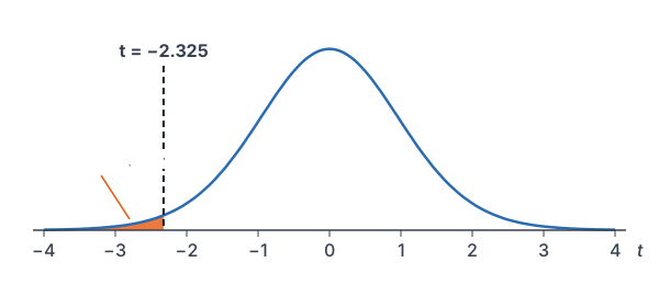
t = \dfrac{-14}{6.021} \approx -2.325

Divide by SE.

\text{df} = 20 - 1 = 19

Use the smaller sample size minus 1.

P(t \le -2.325) = \text{tcdf}(-10^{99}, -2.325, 19)

Find the left-tail area.

\approx 0.0157

Read the calculator result.

0.0157 \lt 0.05

Compare the p-value with α.

Conclude: the p-value is about 0.0157, which is less than 0.05, so reject H₀. There is convincing evidence that caffeine lowers the mean reaction time. Because the groups were randomly assigned, caffeine likely caused the difference.

A t-distribution curve with 19 degrees of freedom on a t axis from −4 to 4. The area to the left of t = −2.325 is shaded orange and labeled p-value ≈ 0.0157. A dashed line marks t = −2.325. — In Example 2, t ≈ −2.325. If caffeine made no difference, a result this extreme would happen only about 1.6% of the time.

Example 3: A two-sided test

A reporter takes random samples of workers in two cities. In City A, 15 workers have a mean commute of 28.4 minutes with s = 7.2. In City B, 12 workers have a mean of 24.9 minutes with s = 5.1. Both samples show no strong skew or outliers. Do the mean commute times differ? Use α = 0.05.

7.2^2 = 51.84

Square s₁.

\dfrac{51.84}{15} = 3.456

Divide by n₁.

5.1^2 = 26.01

Square s₂.

\dfrac{26.01}{12} = 2.1675

Divide by n₂.

3.456 + 2.1675 = 5.6235

Add the two parts.

\text{SE} = \sqrt{5.6235} \approx 2.371

Take the square root.

28.4 - 24.9 = 3.5

Subtract the sample means.

t = \dfrac{3.5}{2.371} \approx 1.476

Divide by SE.

\text{df} = 12 - 1 = 11

Use the smaller sample size minus 1.

P(t \ge 1.476) = \text{tcdf}(1.476, 10^{99}, 11) \approx 0.0840

Find one tail.

2 \cdot 0.0840 = 0.1680

Double it for a two-sided test.

0.1680 \gt 0.05

Compare the p-value with α.

Answer: with H₀: μ₁ = μ₂ and Hₐ: μ₁ ≠ μ₂, the p-value is about 0.168, so fail to reject H₀. The data don’t give convincing evidence that the mean commutes differ. (The TI-84 uses df ≈ 24.7 and gives p ≈ 0.153, which leads to the same conclusion.)

Example 4: Matching a test with an interval

Use the commute data from Example 3. Build a 95% confidence interval for μ₁ − μ₂ with df = 11. Does it agree with the test?

t^* = \text{invT}(0.975, 11) \approx 2.201

Find t* for 95% confidence with df = 11.

\text{ME} = 2.201 \cdot 2.371 \approx 5.219

Multiply t* by SE.

3.5 - 5.219 = -1.719

Subtract ME.

3.5 + 5.219 = 8.719

Add ME.

Answer: about (−1.72, 8.72) minutes. The interval contains 0, so “no difference” is plausible, which matches the test. This is the confidence interval for a difference in means.

Example 5: Checking the conditions

A study compares random samples of house prices in two towns. Town A has 12 prices, and one house costs far more than the rest. Town B has 40 prices with a strong right skew. Can you use a two-sample t-test?

40 \ge 30

Compare n₂ with 30.

12 \lt 30

Compare n₁ with 30.

Answer: Town B is fine because n₂ ≥ 30. Town A is not: its sample is small and has an outlier. Both groups must pass, so the two-sample t-test is not safe here.

Common mistakes

Mistake	Example of the error	Fix
Using a two-sample test on paired data	Comparing before and after scores of the same students as two groups	Use a paired t-test on the differences.
Adding standard deviations instead of variances	SE = √(18/20 + 21/22)	Square each s first: SE = √(18²/20 + 21²/22).
Using n₁ + n₂ − 1 for df	df = 41 for groups of 20 and 22	By hand, use the smaller n minus 1: df = 19.
Claiming cause from an observational study	“Living in City A causes longer commutes.”	Only a randomized experiment supports cause and effect.
Saying “the means are equal” after failing to reject	“The two cities have the same mean commute.”	Say the data don’t give convincing evidence of a difference.

Related methods

Estimating the difference

To estimate how big the difference is, use the confidence interval for a difference in means: (x̄₁ − x̄₂) ± t* · SE.

Comparing proportions instead

If the response is a category (yes or no) rather than a number, compare groups with a two-proportion z-test instead.

Practice problems

Group 1 has s₁ = 4 and n₁ = 16. Group 2 has s₂ = 6 and n₂ = 9. Find the standard error of x̄₁ − x̄₂.
Use Problem 1 with x̄₁ = 50 and x̄₂ = 46. Find t and the conservative df.
Use Problem 2 with Hₐ: μ₁ > μ₂. Find the p-value.
A two-sided two-sample t-test gives t = −2.5 with df = 14. Find the p-value.
Write H₀ and Hₐ to test whether students who sleep 8+ hours have a higher mean GPA than students who sleep less.
Random samples of students who took an exam online (n = 35, x̄ = 78.2, s = 9.5) and in person (n = 40, x̄ = 74.1, s = 11.2) are compared. Test Hₐ: μ₁ ≠ μ₂ at α = 0.05.
In a randomized experiment, a two-sample t-test of a new teaching method gives a p-value of 0.012. Write the conclusion at α = 0.05.
Should you use a two-sample t-test or a paired t-test? (a) Test scores of 30 students before and after a course. (b) Test scores of 30 students in one class and 28 in another.
Why does the two-sample t-test not pool the two standard deviations?
Two random samples have n₁ = 10 and n₂ = 12. Dot plots of both show roughly symmetric data with no outliers. Is the Normal/Large Sample condition met?

Show answers

\dfrac{4^2}{16} = \dfrac{16}{16} = 1

Square s₁ and divide by n₁.

\dfrac{6^2}{9} = \dfrac{36}{9} = 4

Square s₂ and divide by n₂.

1 + 4 = 5

Add the two parts.

\text{SE} = \sqrt{5} \approx 2.236

Take the square root.

Answer: SE ≈ 2.236

50 - 46 = 4

Subtract the sample means.

t = \dfrac{4}{2.236} \approx 1.789

Divide by SE.

\text{df} = 9 - 1 = 8

Use the smaller sample size minus 1.

Answer: t ≈ 1.789 with df = 8

P(t \ge 1.789) = \text{tcdf}(1.789, 10^{99}, 8) \approx 0.0557

Find the right-tail area.

Answer: about 0.0557

P(t \le -2.5) = \text{tcdf}(-10^{99}, -2.5, 14) \approx 0.01273

Find one tail.

2 \cdot 0.01273 \approx 0.0255

Double it for a two-sided test.

Answer: about 0.0255

Answer: H₀: μ₁ = μ₂ and Hₐ: μ₁ > μ₂, where μ₁ and μ₂ are the true mean GPAs of students who sleep 8+ hours and students who sleep less.

\dfrac{9.5^2}{35} = \dfrac{90.25}{35} \approx 2.579

Square s₁ and divide by n₁.

\dfrac{11.2^2}{40} = \dfrac{125.44}{40} = 3.136

Square s₂ and divide by n₂.

2.579 + 3.136 = 5.715

Add the two parts.

\text{SE} = \sqrt{5.715} \approx 2.391

Take the square root.

78.2 - 74.1 = 4.1

Subtract the sample means.

t = \dfrac{4.1}{2.391} \approx 1.715

Divide by SE.

\text{df} = 35 - 1 = 34

Use the smaller sample size minus 1.

P(t \ge 1.715) = \text{tcdf}(1.715, 10^{99}, 34) \approx 0.0477

Find one tail.

2 \cdot 0.0477 = 0.0954

Double it for a two-sided test.

0.0954 \gt 0.05

Compare with α.

Answer: p-value ≈ 0.095, so fail to reject H₀. The data don’t give convincing evidence that the mean scores differ for online and in-person exams.

0.012 \lt 0.05

Compare the p-value with α.

Answer: Reject H₀. There is convincing evidence that the new method changes the mean score, and because of random assignment, the method likely caused the difference.

Answer: (a) Paired t-test, because each student gives two linked scores. (b) Two-sample t-test, because the two classes are separate groups.

Answer: The two populations may have different spreads. Using each sample’s own s keeps the test accurate when the spreads differ.

10.

Answer: Yes. Both samples are small, but their dot plots show no strong skew or outliers, so the condition is met for each group.

Two-sample t-test FAQ

What is the formula for a two-sample t-test?

The test statistic is t = (x̄₁ − x̄₂) ÷ √(s₁²/n₁ + s₂²/n₂). The p-value comes from a t-distribution with the conservative df (smaller n minus 1) or the calculator’s df.

How do you find degrees of freedom for a two-sample t-test?

By hand, use the smaller of n₁ − 1 and n₂ − 1. Calculators and software use a longer formula (Welch’s) that usually gives a decimal df between that value and n₁ + n₂ − 2.

What is the difference between a two-sample t-test and a paired t-test?

A two-sample t-test compares two independent groups. A paired t-test is for linked pairs, such as before-and-after measurements on the same people, and it works with the differences.

How do you do a 2-SampTTest on a TI-84?

Press STAT, choose TESTS, then 4:2-SampTTest. Enter each group’s x̄, s and n, choose the direction of Hₐ, set Pooled to No, then choose Calculate.

Summary

Use a two-sample t-test to check H₀: μ₁ = μ₂ for two independent groups.
t = (x̄₁ − x̄₂) ÷ √(s₁²/n₁ + s₂²/n₂).
By hand, df = the smaller of n₁ − 1 and n₂ − 1; a calculator uses a more exact df.
Check Random, 10% and Normal/Large Sample for both groups.
Conclude in context. Only a randomized experiment supports cause and effect.

Previous lesson: Paired t-Test

Next lesson: Chi-Square Goodness-of-Fit Test

Back to the Statistics Index