
Chi-Square Goodness-of-Fit Test
A chi-square goodness-of-fit test checks whether the counts in one categorical variable fit a claimed distribution. For each category, compare the observed count O with the expected count E, then add up χ² = Σ (O − E)²/E. Use df = number of categories − 1. A large χ² and a small p-value are evidence that the claim is wrong.
Before this lesson: Categorical and Quantitative Variables, Hypothesis Testing and P-Values
How the test works
Suppose a fruit snack company says its bags are 30% red, 20% blue, 20% green and 30% yellow. You count the colors in a random sample. Your counts will never match the claim exactly. The question is whether they are too far off to blame on chance.
The null hypothesis is the claimed distribution. The expected count for each category is what you’d see on average if H₀ were true: E = n × (claimed proportion). Each term (O − E)²/E measures how far one category is from its expected count, scaled by its size.
Adding the terms gives the chi-square statistic χ². It is never negative. A χ² near 0 means the counts fit the claim well. A large χ² means a poor fit, so the p-value is always the area to the right of χ².
Chi-square goodness-of-fit formula
\chi^2 = \sum \dfrac{(O - E)^2}{E}, \qquad \text{df} = k - 1- O is an observed count, E = n · pᵢ is its expected count, and k is the number of categories.
- H₀: the claimed distribution is correct. Hₐ: the distribution is not as claimed (at least one pᵢ is different).
- The p-value is P(χ² ≥ your value) = χ²cdf(χ², 10^99, df).
- On a TI-84: put the observed counts in L1 and the expected counts in L2. Then STAT, TESTS, D:χ²GOF-Test, enter df and choose Calculate.
Conditions
- Random: the data come from a random sample or a randomized experiment.
- 10%: when sampling without replacement, n is at most 10% of the population.
- Large Counts: every expected count is at least 5.
Chi-square goodness-of-fit examples
Example 1: Find the expected counts
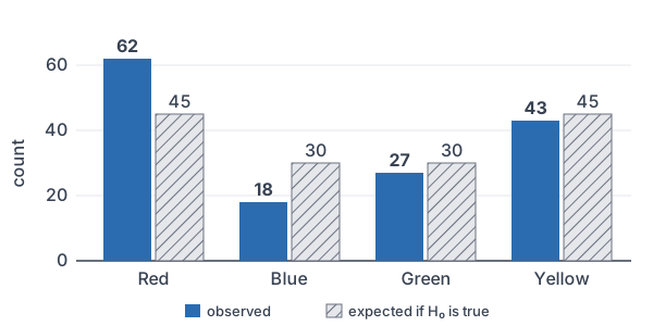
A bag has 150 fruit snacks. The company claims 30% red, 20% blue, 20% green and 30% yellow. Find the expected count for each color.
150 \cdot 0.30 = 45
Expected red: multiply n by 0.30.
150 \cdot 0.20 = 30
Expected blue: multiply n by 0.20.
150 \cdot 0.20 = 30
Expected green.
150 \cdot 0.30 = 45
Expected yellow.
45 + 30 + 30 + 45 = 150
Check that the expected counts add to n.
Answer: 45 red, 30 blue, 30 green and 45 yellow. Expected counts don’t have to be whole numbers.
Example 2: Fruit snack colors (word problem)
A random sample of 150 fruit snacks has 62 red, 18 blue, 27 green and 43 yellow. Do these data give convincing evidence that the company’s color claim is wrong? Use α = 0.05.
State: H₀: the color distribution is 30% red, 20% blue, 20% green, 30% yellow. Hₐ: the distribution is different. Plan: chi-square goodness-of-fit test. The sample is random, 150 is less than 10% of all snacks made, and every expected count from Example 1 is at least 5.
\dfrac{(62 - 45)^2}{45} = \dfrac{289}{45} \approx 6.422Red: square the gap and divide by E.
\dfrac{(18 - 30)^2}{30} = \dfrac{144}{30} = 4.8Blue.
\dfrac{(27 - 30)^2}{30} = \dfrac{9}{30} = 0.3Green.
\dfrac{(43 - 45)^2}{45} = \dfrac{4}{45} \approx 0.089Yellow.
6.422 + 4.8 + 0.3 + 0.089 = 11.611
Add the four terms to get χ².
\text{df} = 4 - 1 = 3Subtract 1 from the number of categories.
P(\chi^2 \ge 11.61) = \chi^2\text{cdf}(11.61, 10^{99}, 3)Find the right-tail area.
\approx 0.0088
Read the calculator result.
0.0088 \lt 0.05
Compare the p-value with α.
Conclude: the p-value is about 0.0088, which is less than 0.05, so reject H₀. There is convincing evidence that the color distribution of the company’s fruit snacks is not 30% red, 20% blue, 20% green and 30% yellow.
Example 3: Is the die fair?
A student rolls a die 120 times and gets these counts for faces 1 through 6: 15, 24, 18, 27, 16 and 20. Is there convincing evidence that the die is unfair? Use α = 0.05.
120 \cdot \dfrac{1}{6} = 20Find the expected count for each face (see multiplying fractions).
\dfrac{(15 - 20)^2}{20} = \dfrac{25}{20} = 1.25Face 1.
\dfrac{(24 - 20)^2}{20} = \dfrac{16}{20} = 0.8Face 2.
\dfrac{(18 - 20)^2}{20} = \dfrac{4}{20} = 0.2Face 3.
\dfrac{(27 - 20)^2}{20} = \dfrac{49}{20} = 2.45Face 4.
\dfrac{(16 - 20)^2}{20} = \dfrac{16}{20} = 0.8Face 5.
\dfrac{(20 - 20)^2}{20} = 0Face 6.
1.25 + 0.8 + 0.2 + 2.45 + 0.8 + 0 = 5.5
Add the terms to get χ².
\text{df} = 6 - 1 = 5Subtract 1 from the number of faces.
P(\chi^2 \ge 5.5) = \chi^2\text{cdf}(5.5, 10^{99}, 5) \approx 0.358Find the right-tail area.
0.358 \gt 0.05
Compare the p-value with α.
Answer: with H₀: each face has probability 1/6, the p-value is about 0.358, so fail to reject H₀. The data don’t give convincing evidence that the die is unfair.
Example 4: When the test can’t be used
A school claims 5% of its 1,000 students walk to school. A random sample of 40 students is taken. Can a chi-square goodness-of-fit test (walk vs. don’t walk) be used?
40 \cdot 0.05 = 2
Find the expected count of walkers.
2 \lt 5
Compare with 5.
Answer: No. The expected count of walkers is only 2, so the Large Counts condition fails. A larger sample (at least 100 students) would fix this.
Example 5: Which category made the difference?
In Example 2, H₀ was rejected. Which colors contributed most to χ², and how?
\dfrac{6.422}{11.611} \approx 0.553Red’s share of χ².
\dfrac{4.8}{11.611} \approx 0.413Blue’s share of χ².
Answer: red (about 55% of χ²) and blue (about 41%) contributed the most. There were more red snacks than expected (62 vs. 45) and fewer blue ones (18 vs. 30). Green and yellow were close to their expected counts.
Common mistakes
| Mistake | Example of the error | Fix |
|---|---|---|
| Using percents instead of counts | O = 41.3% for red | Use counts: O = 62. χ² needs counts, not percents. |
| Dividing by O instead of E | (62 − 45)²/62 | Divide by the expected count: (62 − 45)²/45. |
| Checking Large Counts with observed counts | “Blue has 18, so it’s fine.” | Check that every expected count is at least 5. |
| Using df = number of observations − 1 | df = 150 − 1 = 149 | df = number of categories − 1 = 3. |
| Using a two-tailed p-value | Doubling the right-tail area | A χ² test is always right-tailed. |
Related methods
Two categorical variables
A goodness-of-fit test uses one categorical variable and one claimed distribution. To test whether two categorical variables are related in a two-way table, use the chi-square test for independence, the next lesson.
Two categories only
With just two categories, the goodness-of-fit test gives the same p-value as a two-sided one-proportion z-test, because χ² = z².
Practice problems
- A sample of 200 is tested against the claim 50%, 30% and 20% for three categories. Find the expected counts.
- One category has O = 48 and E = 40. Find its term (O − E)²/E.
- A goodness-of-fit test has 7 categories. Find df.
- A test gives χ² = 9.2 with df = 4. Find the p-value.
- A hospital wants to test whether births are spread evenly over the 7 days of the week. Write H₀ and Hₐ.
- A teacher says grades are 20% A, 30% B, 35% C and 15% D or F. In a random sample of 80 grades, there are 22 A’s, 20 B’s, 28 C’s and 10 D/F’s. Test the claim at α = 0.05.
- A claim gives one category a proportion of 0.07, and the sample size is 50. Is the Large Counts condition met?
- A goodness-of-fit test about ice-cream flavor preferences gives a p-value of 0.003 with α = 0.05. Write the conclusion.
- Why is the p-value of a χ² test always the right tail?
- Use Problem 6. Which grade contributed most to χ², and what does it say?
Show answers
1.
200 \cdot 0.5 = 100
First category.
200 \cdot 0.3 = 60
Second category.
200 \cdot 0.2 = 40
Third category.
Answer: 100, 60 and 40
2.
48 - 40 = 8
Subtract E from O.
8^2 = 64
Square the gap.
\dfrac{64}{40} = 1.6Divide by E.
Answer: 1.6
3.
\text{df} = 7 - 1 = 6Subtract 1 from the number of categories.
Answer: df = 6
4.
P(\chi^2 \ge 9.2) = \chi^2\text{cdf}(9.2, 10^{99}, 4) \approx 0.0563Find the right-tail area.
Answer: about 0.0563
5.
Answer: H₀: each day of the week has probability 1/7 of a birth. Hₐ: the days do not all have probability 1/7.
6.
80 \cdot 0.20 = 16
Expected A’s.
80 \cdot 0.30 = 24
Expected B’s.
80 \cdot 0.35 = 28
Expected C’s.
80 \cdot 0.15 = 12
Expected D/F’s.
\dfrac{(22 - 16)^2}{16} = \dfrac{36}{16} = 2.25A term.
\dfrac{(20 - 24)^2}{24} = \dfrac{16}{24} \approx 0.667B term.
\dfrac{(28 - 28)^2}{28} = 0C term.
\dfrac{(10 - 12)^2}{12} = \dfrac{4}{12} \approx 0.333D/F term.
2.25 + 0.667 + 0 + 0.333 = 3.25
Add the terms to get χ².
\text{df} = 4 - 1 = 3Subtract 1 from the number of categories.
P(\chi^2 \ge 3.25) = \chi^2\text{cdf}(3.25, 10^{99}, 3) \approx 0.355Find the right-tail area.
0.355 \gt 0.05
Compare with α.
Answer: p-value ≈ 0.355, so fail to reject H₀. The data don’t give convincing evidence that the grade distribution differs from the teacher’s claim.
7.
50 \cdot 0.07 = 3.5
Find the expected count.
3.5 \lt 5
Compare with 5.
Answer: No. The expected count 3.5 is less than 5.
8.
0.003 \lt 0.05
Compare the p-value with α.
Answer: Reject H₀. There is convincing evidence that the flavor preferences are not distributed as claimed.
9.
Answer: Each term (O − E)²/E is 0 or positive, so χ² grows as the fit gets worse. Only large values count as evidence against H₀, so the p-value is the area to the right.
10.
Answer: The A term, 2.25, is the largest. There were more A’s than expected (22 vs. 16).
Chi-square goodness-of-fit FAQ
What is the formula for a chi-square goodness-of-fit test?
The test statistic is χ² = Σ (O − E)²/E, added over all categories, with df = number of categories − 1. The expected count for each category is E = n times the claimed proportion.
How do you find expected counts?
Multiply the sample size n by the claimed proportion for each category. For a fair die rolled 120 times, each face has E = 120 × 1/6 = 20.
What are the conditions for a chi-square goodness-of-fit test?
The data must come from a random sample or experiment, the sample must be at most 10% of the population, and every expected count must be at least 5.
How do you do a χ²GOF-Test on a TI-84?
Enter the observed counts in L1 and the expected counts in L2. Press STAT, choose TESTS, then D:χ²GOF-Test. Enter Observed: L1, Expected: L2 and df, then choose Calculate.
Summary
- Use a chi-square goodness-of-fit test to check a claimed distribution for one categorical variable.
- Expected count: E = n × claimed proportion.
- χ² = Σ (O − E)²/E, with df = number of categories − 1.
- Check Random, 10% and Large Counts (every expected count at least 5).
- The p-value is always the right tail. Look at the largest terms to see which categories differ most.
Previous lesson: Two-Sample t-Test
Next lesson: Chi-Square Test for Independence
Back to the Statistics Index