
One-Proportion z-Test
A one-proportion z-test checks a claim about a single population proportion p. You compare the sample proportion p̂ with the claimed value p₀ using z = (p̂ − p₀) ÷ √(p₀(1 − p₀)/n). Then you find the p-value from the normal curve. A small p-value is evidence against the claim.
Before this lesson: Hypothesis Testing, P-Values and Sampling Distribution of a Sample Proportion
How the test works
Suppose a school says 70% of its students eat breakfast. If that claim is true, sample proportions from random samples pile up around 0.70 in a roughly normal shape. Its spread is the standard error √(p₀(1 − p₀)/n).
The z statistic says how many standard errors your p̂ is from p₀. A z far from 0 means your sample would be unusual if the claim were true. The p-value turns that distance into a probability.
Notice that the standard error uses p₀, not p̂. A test assumes H₀ is true, so it uses the claimed value. (A confidence interval for a proportion uses p̂ instead, because it has no claimed value.)
One-proportion z-test formula
z = \dfrac{\hat{p} - p_0}{\sqrt{\dfrac{p_0(1 - p_0)}{n}}}- H₀: p = p₀, and Hₐ is p > p₀, p < p₀ or p ≠ p₀.
- The p-value is the tail area beyond z that matches Hₐ (both tails for ≠).
- On a TI-84: STAT, TESTS, 5:1-PropZTest. Enter p₀, x (the count of successes), n, and the direction of Hₐ.
Conditions
- Random: the data come from a random sample or a randomized experiment.
- 10%: when sampling without replacement, n is at most 10% of the population.
- Large Counts: np₀ ≥ 10 and n(1 − p₀) ≥ 10. Use p₀, the null value, for this check.
One-proportion z-test examples
Example 1: Breakfast survey (word problem)
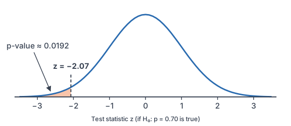
A school claims 70% of its students eat breakfast. The nurse thinks the rate is lower. In a random sample of 250 students, 160 ate breakfast. Test at α = 0.05.
State: H₀: p = 0.70 and Hₐ: p < 0.70, where p is the proportion of all students at the school who eat breakfast. Plan: one-proportion z-test. The sample is random, 250 is less than 10% of a large school, and the counts below are at least 10.
250 \cdot 0.70 = 175
Check np₀ ≥ 10.
250 \cdot 0.30 = 75
Check n(1 − p₀) ≥ 10.
\hat{p} = \dfrac{160}{250} = 0.64Divide successes by n.
0.70 \cdot 0.30 = 0.21
Multiply p₀(1 − p₀).
\dfrac{0.21}{250} = 0.00084Divide by n.
\text{SE} = \sqrt{0.00084} \approx 0.02898Take the square root (see square roots).
0.64 - 0.70 = -0.06
Subtract p₀ from p̂.
z = \dfrac{-0.06}{0.02898} \approx -2.070Divide by SE.
P(Z \le -2.070) = \text{normalcdf}(-10^{99}, -2.070)Find the left-tail area.
\approx 0.0192
Read the calculator result.
0.0192 \lt 0.05
Compare the p-value with α.
Conclude: the p-value is about 0.0192, which is less than 0.05, so reject H₀. There is convincing evidence that fewer than 70% of the school’s students eat breakfast.
Example 2: A two-sided test
A spinner is supposed to land on red 25% of the time. In 400 spins it lands on red 116 times. Test H₀: p = 0.25 against Hₐ: p ≠ 0.25 at α = 0.05.
\hat{p} = \dfrac{116}{400} = 0.29Divide red spins by n.
0.25 \cdot 0.75 = 0.1875
Multiply p₀(1 − p₀).
\dfrac{0.1875}{400} = 0.00046875Divide by n.
\text{SE} = \sqrt{0.00046875} \approx 0.02165Take the square root.
0.29 - 0.25 = 0.04
Subtract p₀ from p̂.
z = \dfrac{0.04}{0.02165} \approx 1.848Divide by SE.
P(Z \ge 1.848) \approx 0.0323
One tail, from normalcdf(1.848, 10^99).
2 \cdot 0.0323 = 0.0646
Double it for a two-sided test.
0.0646 \gt 0.05
Compare the p-value with α.
Answer: the p-value is about 0.0646, so fail to reject H₀. The data don’t give convincing evidence that the spinner’s red rate differs from 25%. Counts check: 400 · 0.25 = 100 and 400 · 0.75 = 300.
Example 3: Same data, stricter α
A city council member claims more than half of voters support a new park. In a random sample of 1,000 voters, 532 support it. Test at α = 0.01.
\hat{p} = \dfrac{532}{1000} = 0.532Divide supporters by n.
\dfrac{0.5 \cdot 0.5}{1000} = \dfrac{0.25}{1000}Multiply p₀(1 − p₀).
= 0.00025
Divide by n.
\text{SE} = \sqrt{0.00025} \approx 0.01581Take the square root.
z = \dfrac{0.532 - 0.5}{0.01581} = \dfrac{0.032}{0.01581}Subtract p₀ from p̂.
\approx 2.024
Divide by SE.
P(Z \ge 2.024) = \text{normalcdf}(2.024, 10^{99})Find the right-tail area.
\approx 0.0215
Read the calculator result.
0.0215 \gt 0.01
Compare the p-value with α = 0.01.
Answer: with H₀: p = 0.5 and Hₐ: p > 0.5, the p-value is about 0.0215. That is above 0.01, so fail to reject H₀ at this strict level. At α = 0.05, the same data would lead to rejecting H₀.
Example 4: When the test can’t be used
A company claims only 10% of its phones need repairs in the first year. A reviewer checks a random sample of 40 phones. Can the reviewer use a one-proportion z-test?
40 \cdot 0.10 = 4
Find np₀.
4 \lt 10
Compare with 10.
Answer: No. The expected count of repairs is only 4, so the Large Counts condition fails and the normal curve is not a good model. The reviewer needs a larger sample (at least 100 phones) or an exact binomial method (see the binomial distribution).
Example 5: Matching a test with an interval
Use the spinner data from Example 2 (p̂ = 0.29, n = 400). Build a 95% confidence interval for p. Does it agree with the test?
0.29 \cdot 0.71 = 0.2059
Multiply p̂(1 − p̂); intervals use p̂.
\dfrac{0.2059}{400} = 0.00051475Divide by n.
\text{SE} = \sqrt{0.00051475} \approx 0.02269Take the square root.
\text{ME} = 1.96 \cdot 0.02269 \approx 0.0445Multiply z* = 1.96 by SE.
0.29 - 0.0445 = 0.2455
Subtract ME.
0.29 + 0.0445 = 0.3345
Add ME.
Answer: about (0.246, 0.335). The claimed value 0.25 is inside the interval, so it is plausible. That matches the test, which failed to reject H₀: p = 0.25.
Common mistakes
| Mistake | Example of the error | Fix |
|---|---|---|
| Using p̂ in the test’s standard error | SE = √(0.64 · 0.36/250) | Use p₀: SE = √(0.70 · 0.30/250). |
| Checking Large Counts with p̂ | 160 and 90 for the breakfast data | Use p₀: 175 and 75. |
| Not doubling a two-sided p-value | Reporting 0.0323 for Hₐ: p ≠ 0.25 | Two-sided p-value = 2 × 0.0323 = 0.0646. |
| Entering p̂ instead of x in 1-PropZTest | x: 0.64 | Enter the count, x = 160. |
| Concluding about the sample | “64% of the sample eat breakfast, so reject” | Conclude about p, the proportion of all students. |
Related methods
Comparing two groups
To test whether two population proportions differ, use a two-proportion z-test. Its interval version is the confidence interval for a difference in proportions.
Errors in decisions
Any test can reach the wrong decision by chance. The next lesson, Type I and Type II Errors, explains the two kinds of mistakes and what power means.
Practice problems
- A test uses p₀ = 0.08 and n = 150. Is the Large Counts condition met?
- Find the standard error for a test with p₀ = 0.4 and n = 600.
- Use Problem 2. A sample gives p̂ = 0.43. Find z.
- Use Problem 3 with Hₐ: p > 0.4. Find the p-value.
- A two-sided test gives z = −2.4. Find the p-value.
- Test H₀: p = 0.5 against Hₐ: p > 0.5 when 61 of 100 randomly chosen people say yes. Use α = 0.05.
- Why does a one-proportion z-test use p₀ in the standard error?
- A test of a company’s claim that 30% of customers are repeat buyers gives p-value = 0.08 with α = 0.05. Write the conclusion.
- A test uses p₀ = 0.15 with n = 50. Can you use a one-proportion z-test?
- A store claims 90% of orders ship on time. In a random sample of 200 orders, 172 shipped on time. Test Hₐ: p < 0.9 at α = 0.05.
Show answers
1.
150 \cdot 0.08 = 12
Find np₀.
150 \cdot 0.92 = 138
Find n(1 − p₀).
Answer: Yes. Both 12 and 138 are at least 10.
2.
0.4 \cdot 0.6 = 0.24
Multiply p₀(1 − p₀).
\dfrac{0.24}{600} = 0.0004Divide by n.
\text{SE} = \sqrt{0.0004} = 0.02Take the square root.
Answer: SE = 0.02
3.
0.43 - 0.4 = 0.03
Subtract p₀ from p̂.
z = \dfrac{0.03}{0.02} = 1.5Divide by SE.
Answer: z = 1.5
4.
P(Z \ge 1.5) = \text{normalcdf}(1.5, 10^{99})Right-tail area.
\approx 0.0668
Read the calculator result.
Answer: about 0.0668
5.
P(Z \le -2.4) = \text{normalcdf}(-10^{99}, -2.4)One tail.
\approx 0.0082
Read the calculator result.
2 \cdot 0.0082 = 0.0164
Double it for a two-sided test.
Answer: about 0.0164
6.
\hat{p} = \dfrac{61}{100} = 0.61Divide by n.
\dfrac{0.5 \cdot 0.5}{100} = \dfrac{0.25}{100}Multiply p₀(1 − p₀).
= 0.0025
Divide by n.
\text{SE} = \sqrt{0.0025} = 0.05Take the square root.
z = \dfrac{0.61 - 0.5}{0.05} = \dfrac{0.11}{0.05}Subtract p₀ from p̂.
= 2.2
Divide by SE.
P(Z \ge 2.2) = \text{normalcdf}(2.2, 10^{99})Right-tail area.
\approx 0.0139
Read the calculator result.
0.0139 \lt 0.05
Compare with α.
Answer: p-value ≈ 0.0139, so reject H₀. There is convincing evidence that more than half say yes.
7.
The test assumes H₀ is true, so the sampling distribution of p̂ is centered at p₀ with spread based on p₀.
Answer: because the p-value is computed in a world where p = p₀
8.
0.08 \gt 0.05
Compare the p-value with α.
Answer: Fail to reject H₀. The data don’t give convincing evidence that the proportion of repeat buyers differs from 30%.
9.
50 \cdot 0.15 = 7.5
Find np₀.
7.5 \lt 10
Compare with 10.
Answer: No. np₀ = 7.5 is less than 10, so Large Counts fails.
10.
\hat{p} = \dfrac{172}{200} = 0.86Divide by n.
\dfrac{0.9 \cdot 0.1}{200} = \dfrac{0.09}{200}Multiply p₀(1 − p₀).
= 0.00045
Divide by n.
\text{SE} = \sqrt{0.00045} \approx 0.02121Take the square root.
z = \dfrac{0.86 - 0.9}{0.02121} = \dfrac{-0.04}{0.02121}Subtract p₀ from p̂.
\approx -1.886
Divide by SE.
P(Z \le -1.886) = \text{normalcdf}(-10^{99}, -1.886)Left-tail area.
\approx 0.0296
Read the calculator result.
0.0296 \lt 0.05
Compare with α.
Answer: p-value ≈ 0.0296, so reject H₀. There is convincing evidence that fewer than 90% of orders ship on time. (Counts: 180 and 20 are both at least 10.)
One-proportion z-test FAQ
What is the formula for a one-proportion z-test?
The test statistic is z = (p̂ − p₀) ÷ √(p₀(1 − p₀)/n), where p₀ is the claimed proportion. The p-value is the matching tail area under the standard normal curve.
What are the conditions for a one-proportion z-test?
The data must come from a random sample or experiment, the sample must be at most 10% of the population, and both np₀ and n(1 − p₀) must be at least 10.
How do you do a 1-PropZTest on a TI-84?
Press STAT, choose TESTS, then 5:1-PropZTest. Enter p₀, the number of successes x, the sample size n, and the direction of Hₐ, then choose Calculate.
What is the difference between a one-proportion z-test and a z-interval?
The test checks one claimed value p₀ and uses p₀ in the standard error. The interval estimates p and uses p̂ in the standard error.
Summary
- Use a one-proportion z-test to check a claim H₀: p = p₀.
- z = (p̂ − p₀) ÷ √(p₀(1 − p₀)/n), with p₀ in the standard error.
- Check Random, 10% and Large Counts (np₀ ≥ 10 and n(1 − p₀) ≥ 10).
- Find the p-value in the tail that matches Hₐ, and compare it with α.
- State the conclusion in context about the population proportion p.
Previous lesson: P-Values
Next lesson: Type I and Type II Errors
Back to the Statistics Index