
Confidence Interval for a Difference in Proportions
A confidence interval for a difference in proportions estimates p₁ − p₂, the gap between two population proportions. You build a two-proportion z-interval: (p̂₁ − p̂₂) ± z* times the standard error. If the whole interval is above or below 0, the data show a real difference between the two groups.
Before this lesson: Confidence Interval for a Proportion and Sampling Distributions for Differences
Comparing two groups
Many questions compare two groups. Do more juniors than seniors support a later start time? Does a new treatment cut the infection rate? Each group has its own true proportion, p₁ and p₂.
The difference in sample proportions, p̂₁ − p̂₂, is the point estimate. Its standard error combines the variability of both samples. The variances add, even though the proportions are subtracted, because each sample brings its own random error (see combining random variables).
The key question is whether 0 is inside the interval. A difference of 0 means the two proportions are equal.
Confidence interval for a difference in proportions formula
(\hat{p}_1 - \hat{p}_2) \pm z^* \sqrt{\dfrac{\hat{p}_1(1 - \hat{p}_1)}{n_1} + \dfrac{\hat{p}_2(1 - \hat{p}_2)}{n_2}}- p̂₁ and p̂₂ are the sample proportions, and n₁ and n₂ are the sample sizes.
- The square root is the standard error (SE) of p̂₁ − p̂₂.
- z* is 1.645 for 90%, 1.96 for 95% and 2.576 for 99%.
- The margin of error is ME = z* · SE.
Conditions
- Random: two independent random samples, or two groups in a randomized experiment.
- 10%: when sampling without replacement, each sample is at most 10% of its population. (Not needed for an experiment.)
- Large Counts: n₁p̂₁, n₁(1 − p̂₁), n₂p̂₂ and n₂(1 − p̂₂) are all at least 10.
Calculator: on a TI-84, press STAT, choose TESTS, then B:2-PropZInt. Enter the success counts x₁ and x₂, the sample sizes n₁ and n₂, and the C-Level.
Reading the interval
| Interval for p₁ − p₂ | What it means |
|---|---|
| All values above 0 | p₁ is larger than p₂. |
| All values below 0 | p₁ is smaller than p₂. |
| Contains 0 | No convincing difference; equal proportions are plausible. |
Confidence interval for a difference in proportions examples
Example 1: Survey of two grades (word problem)
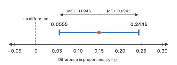
A school asks random samples of students whether they support a later start time. Of 200 juniors, 120 say yes. Of 220 seniors, 99 say yes. Build a 95% confidence interval for p₁ − p₂, where 1 = juniors and 2 = seniors.
Conditions: both samples are random and independent, each is less than 10% of a large grade, and the counts 120, 80, 99 and 121 are all at least 10.
\hat{p}_1 = \dfrac{120}{200} = 0.60Divide yes answers by n₁.
\hat{p}_2 = \dfrac{99}{220} = 0.45Divide yes answers by n₂.
0.60 - 0.45 = 0.15
Subtract to get the point estimate.
0.60 \cdot 0.40 = 0.24
Find p̂₁(1 − p̂₁).
\dfrac{0.24}{200} = 0.0012Divide by n₁.
0.45 \cdot 0.55 = 0.2475
Find p̂₂(1 − p̂₂).
\dfrac{0.2475}{220} = 0.001125Divide by n₂.
0.0012 + 0.001125 = 0.002325
Add the two variances.
\text{SE} = \sqrt{0.002325} \approx 0.04822Take the square root (see square roots).
\text{ME} = 1.96 \cdot 0.04822 \approx 0.0945Multiply z* by SE.
0.15 - 0.0945 = 0.0555
Subtract ME from the estimate.
0.15 + 0.0945 = 0.2445
Add ME to the estimate.
Answer: about (0.056, 0.245). We are 95% confident that the share of juniors who support a later start is between 5.6 and 24.5 percentage points higher than the share of seniors. The whole interval is above 0, so juniors are more supportive.
Example 2: An interval that contains 0
A gardener plants random samples of two seed brands. Brand A: 84 of 120 seeds sprout. Brand B: 78 of 120 sprout. Build a 90% confidence interval for p_A - p_B.
\hat{p}_A = \dfrac{84}{120} = 0.70Divide by n for brand A.
\hat{p}_B = \dfrac{78}{120} = 0.65Divide by n for brand B.
0.70 - 0.65 = 0.05
Subtract to get the point estimate.
\dfrac{0.70 \cdot 0.30}{120} = \dfrac{0.21}{120}Multiply p̂(1 − p̂) for brand A.
= 0.00175
Divide by 120.
\dfrac{0.65 \cdot 0.35}{120} = \dfrac{0.2275}{120}Multiply p̂(1 − p̂) for brand B.
\approx 0.001896
Divide by 120.
0.00175 + 0.001896 = 0.003646
Add the two variances.
\text{SE} = \sqrt{0.003646} \approx 0.06038Take the square root.
\text{ME} = 1.645 \cdot 0.06038 \approx 0.0993Multiply z* = 1.645 by SE.
0.05 - 0.0993 = -0.0493
Subtract ME from the estimate.
0.05 + 0.0993 = 0.1493
Add ME to the estimate.
Answer: about (−0.049, 0.149). The interval contains 0, so the data don’t give convincing evidence that one brand sprouts more often. Brand A could be up to 14.9 points better or up to 4.9 points worse.
Example 3: A randomized experiment at 99%
In an experiment, 1,000 volunteers are randomly assigned to a new flu shot or a placebo, 500 each. In the shot group, 30 get the flu. In the placebo group, 55 get the flu. Build a 99% confidence interval for p_{\text{shot}} - p_{\text{placebo}}.
Conditions: random assignment; the 10% condition is not needed for an experiment; the counts 30, 470, 55 and 445 are all at least 10.
\hat{p}_1 = \dfrac{30}{500} = 0.06Flu rate for the shot group.
\hat{p}_2 = \dfrac{55}{500} = 0.11Flu rate for the placebo group.
0.06 - 0.11 = -0.05
Subtract to get the point estimate.
\dfrac{0.06 \cdot 0.94}{500} = \dfrac{0.0564}{500}Multiply p̂(1 − p̂) for the shot group.
= 0.0001128
Divide by 500.
\dfrac{0.11 \cdot 0.89}{500} = \dfrac{0.0979}{500}Multiply p̂(1 − p̂) for the placebo group.
= 0.0001958
Divide by 500.
0.0001128 + 0.0001958 = 0.0003086
Add the two variances.
\text{SE} = \sqrt{0.0003086} \approx 0.01757Take the square root.
\text{ME} = 2.576 \cdot 0.01757 \approx 0.04526Multiply z* = 2.576 by SE.
-0.05 - 0.04526 = -0.09526
Subtract ME from the estimate.
-0.05 + 0.04526 = -0.00474
Add ME to the estimate.
Answer: about (−0.095, −0.005). The whole interval is below 0, so the flu rate is lower with the shot. Because this was a randomized experiment, the shot can be credited with the drop.
Example 4: When the conditions fail
A random sample of 50 phone users finds 4 who use a certain app. A random sample of 60 tablet users finds 12. Can you build a two-proportion z-interval?
50 \cdot 0.08 = 4
Count of successes for phones, with p̂₁ = 4/50 = 0.08.
4 \lt 10
Compare with 10.
Answer: No. Only 4 phone users are successes, which is fewer than 10, so the Large Counts condition fails. The normal approximation is not reliable, and the interval could be misleading.
Example 5: Read calculator output
2-PropZInt gives the 95% interval (−0.012, 0.108) for p₁ − p₂. Find the point estimate and the margin of error, then interpret the interval.
\dfrac{-0.012 + 0.108}{2} = \dfrac{0.096}{2}Add the endpoints.
= 0.048
Divide by 2; the estimate is the midpoint.
\text{ME} = 0.108 - 0.048 = 0.06Subtract the estimate from the upper endpoint.
Answer: p̂₁ − p̂₂ = 0.048 and ME = 0.06. The interval contains 0, so a difference of 0 is plausible. The data don’t show a convincing difference between the two proportions.
Common mistakes
| Mistake | Example of the error | Fix |
|---|---|---|
| Subtracting the variances | 0.0012 − 0.001125 under the square root | Always add: SE = √(0.0012 + 0.001125). |
| Using one combined n | Dividing both parts by 420 | Divide each part by its own sample size. |
| Forgetting which order you subtracted | Reading (0.056, 0.245) as “seniors are higher” | Define p₁ − p₂ in words before you compute. |
| Skipping Large Counts | Building an interval with only 4 successes | Check all four counts are at least 10. |
| Saying 0 in the interval proves no difference | “The brands sprout at the same rate” | Say the data don’t show a convincing difference. |
Related methods
Testing a difference
A confidence interval estimates how big the gap is. A two-proportion z-test asks whether any gap exists. An interval that leaves out 0 points the same way as a test that rejects “no difference.”
Means instead of proportions
For a difference in two means, you use a two-sample t-interval instead. The next lesson, Confidence Interval for a Difference in Means, shows how.
Practice problems
- In one sample, 45 of 75 say yes. In another, 30 of 60 say yes. Find p̂₁, p̂₂ and p̂₁ − p̂₂.
- Find the SE of p̂₁ − p̂₂ when p̂₁ = 0.5 with n₁ = 100 and p̂₂ = 0.4 with n₂ = 150.
- Use Problem 2. Build a 95% confidence interval for p₁ − p₂.
- Sample 1 has 12 successes out of 80. Sample 2 has 6 successes out of 50. Is the Large Counts condition met?
- A 95% interval for p₁ − p₂ is (0.02, 0.11). Interpret it.
- A 95% interval for p₁ − p₂ is (−0.07, 0.04). Do the data show a difference?
- 2-PropZInt gives (0.031, 0.149). Find the point estimate and the margin of error.
- An interval for p₁ − p₂ is (0.03, 0.12). What is the interval for p₂ − p₁?
- In random samples, 66 of 150 city voters and 50 of 125 rural voters back a plan. Build a 90% interval for p_{\text{city}} - p_{\text{rural}}.
- If both sample sizes are multiplied by 4 and the sample proportions stay the same, what happens to the margin of error?
Show answers
1.
\hat{p}_1 = \dfrac{45}{75} = 0.6Divide 45 by 75.
\hat{p}_2 = \dfrac{30}{60} = 0.5Divide 30 by 60.
0.6 - 0.5 = 0.1
Subtract.
Answer: p̂₁ = 0.6, p̂₂ = 0.5 and p̂₁ − p̂₂ = 0.1
2.
\dfrac{0.5 \cdot 0.5}{100} = \dfrac{0.25}{100}Multiply p̂₁(1 − p̂₁).
= 0.0025
Divide by 100.
\dfrac{0.4 \cdot 0.6}{150} = \dfrac{0.24}{150}Multiply p̂₂(1 − p̂₂).
= 0.0016
Divide by 150.
0.0025 + 0.0016 = 0.0041
Add the variances.
\text{SE} = \sqrt{0.0041} \approx 0.06403Take the square root.
Answer: SE ≈ 0.064
3.
0.5 - 0.4 = 0.1
Find the point estimate.
\text{ME} = 1.96 \cdot 0.06403 \approx 0.1255Multiply z* by SE.
0.1 - 0.1255 = -0.0255
Subtract ME.
0.1 + 0.1255 = 0.2255
Add ME.
Answer: about (−0.026, 0.226)
4.
6 \lt 10
Sample 2 has only 6 successes.
Answer: No. Sample 2 has fewer than 10 successes, so the condition fails.
5.
Both endpoints are above 0.
Answer: We are 95% confident that p₁ is between 2 and 11 percentage points higher than p₂. The data show p₁ is larger.
6.
The interval contains 0.
Answer: No. A difference of 0 is plausible, so the data don’t show a convincing difference.
7.
\dfrac{0.031 + 0.149}{2} = \dfrac{0.18}{2}Add the endpoints.
= 0.09
Divide by 2.
\text{ME} = 0.149 - 0.09 = 0.059Subtract the estimate from the upper endpoint.
Answer: estimate 0.09, ME = 0.059
8.
Switching the order changes every sign, and the endpoints swap places.
Answer: (−0.12, −0.03)
9.
\hat{p}_1 = \dfrac{66}{150} = 0.44City proportion.
\hat{p}_2 = \dfrac{50}{125} = 0.40Rural proportion.
0.44 - 0.40 = 0.04
Point estimate.
\dfrac{0.44 \cdot 0.56}{150} = \dfrac{0.2464}{150}Multiply p̂₁(1 − p̂₁).
\approx 0.001643
Divide by 150.
\dfrac{0.40 \cdot 0.60}{125} = \dfrac{0.24}{125}Multiply p̂₂(1 − p̂₂).
= 0.00192
Divide by 125.
0.001643 + 0.00192 = 0.003563
Add the variances.
\text{SE} = \sqrt{0.003563} \approx 0.05969Take the square root.
\text{ME} = 1.645 \cdot 0.05969 \approx 0.0982Multiply z* = 1.645 by SE.
0.04 - 0.0982 = -0.0582
Subtract ME.
0.04 + 0.0982 = 0.1382
Add ME.
Answer: about (−0.058, 0.138). It contains 0, so no convincing difference.
10.
Each variance is divided by a sample size 4 times as big, so the sum of the variances is 1/4 as big. The square root of 1/4 is 1/2.
Answer: The margin of error is cut in half.
Confidence interval for a difference in proportions FAQ
What is the formula for a confidence interval for the difference in two proportions?
It is (p̂₁ − p̂₂) ± z* √(p̂₁(1 − p̂₁)/n₁ + p̂₂(1 − p̂₂)/n₂). The square root is the standard error, and z* depends on the confidence level.
What does it mean if a confidence interval for p₁ − p₂ contains 0?
It means a difference of 0 is plausible, so the data don’t give convincing evidence that the two proportions differ. It does not prove they are equal.
What are the conditions for a two-proportion z-interval?
You need two independent random samples or a randomized experiment, each sample at most 10% of its population, and at least 10 successes and 10 failures in each group.
Does the order of subtraction matter?
The order changes only the signs. An interval of (0.03, 0.12) for p₁ − p₂ is the same result as (−0.12, −0.03) for p₂ − p₁, so state which group is which.
Summary
- The interval is (p̂₁ − p̂₂) ± z* · SE, where SE = √(p̂₁(1 − p̂₁)/n₁ + p̂₂(1 − p̂₂)/n₂).
- Add the two variances under the square root, even though the proportions are subtracted.
- Check Random, 10% and Large Counts (four counts of at least 10).
- An interval entirely above or below 0 shows a real difference; one that contains 0 does not.
- On a TI-84, use 2-PropZInt.
Previous lesson: Confidence Interval for a Mean
Next lesson: Confidence Interval for a Difference in Means
Back to the Statistics Index