
Confidence Interval for a Proportion
A confidence interval for a proportion estimates a population proportion p from a random sample. The formula is \hat{p} \pm z^*\sqrt{\hat{p}(1 - \hat{p})/n}, where p̂ is the sample proportion and z* sets the confidence level. It is also called a one-proportion z-interval.
Before this lesson: Confidence Intervals and Sampling Distribution of a Sample Proportion
How the interval for a proportion works
In the sampling distribution of p̂, the standard deviation is \sqrt{p(1 - p)/n}. But when you build an interval, you don’t know p. That is the whole reason for the interval.
So you use p̂ in its place. The result is the standard error of p̂, an estimate of how far p̂ typically lands from p. Then you reach out z* standard errors on each side of p̂.
Confidence interval for a proportion formula
\hat{p} \pm z^* \sqrt{\dfrac{\hat{p}(1 - \hat{p})}{n}}| Confidence level | 90% | 95% | 99% |
|---|---|---|---|
| z* | 1.645 | 1.960 | 2.576 |
Check three conditions before you use the formula:
- Random: the data come from a random sample.
- 10% condition: n is less than 10% of the population.
- Large Counts: the numbers of successes and failures, n\hat{p} and n(1 - \hat{p}), are both at least 10.
A full answer has four parts: state the parameter and level, name the method and check conditions, do the math, and conclude in context.
Calculator: on a TI-84, press STAT, go to TESTS and choose 1-PropZInt. Enter x (the number of successes), n and the C-Level. It gives the interval directly.
Confidence interval for a proportion examples
Example 1: A 95% interval, all four steps
In a random sample of 600 U.S. teens, 312 say they have used an AI tool for homework. Build a 95% confidence interval for the proportion of all U.S. teens who have done this.
State: p is the proportion of all U.S. teens who have used AI for homework, at 95% confidence. Plan: a one-proportion z-interval. The sample is random, and 600 is far less than 10% of all teens.
312 \ge 10 \text{ and } 600 - 312 = 288 \ge 10Large Counts: successes and failures are both at least 10.
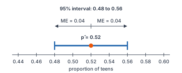
\hat{p} = \dfrac{312}{600} = 0.52Find the sample proportion.
0.52(0.48) = 0.2496
Multiply p̂ by 1 − p̂.
\dfrac{0.2496}{600} = 0.000416Divide by n.
\text{SE} = \sqrt{0.000416} \approx 0.0204Take the square root (see square roots).
\text{ME} = 1.96(0.0204) \approx 0.0400Multiply by z* = 1.96.
0.52 - 0.0400 = 0.48
Lower endpoint.
0.52 + 0.0400 = 0.56
Upper endpoint.
Conclude: we are 95% confident that the interval from 0.48 to 0.56 captures the true proportion of U.S. teens who have used an AI tool for homework.
Example 2: A 90% interval
In a random sample of 150 voters from a town of 8,000, 45 want a new library. Build a 90% confidence interval for the proportion of all the town’s voters who want one.
150 \lt 800
10% condition: 10% of 8,000 is 800.
45 \ge 10 \text{ and } 105 \ge 10Large Counts: 45 successes and 150 − 45 = 105 failures.
\hat{p} = \dfrac{45}{150} = 0.30Find the sample proportion.
0.30(0.70) = 0.21
Multiply p̂ by 1 − p̂.
\dfrac{0.21}{150} = 0.0014Divide by n.
\text{SE} = \sqrt{0.0014} \approx 0.0374Take the square root.
\text{ME} = 1.645(0.0374) \approx 0.0615Multiply by z* = 1.645.
0.30 - 0.0615 = 0.2385
Lower endpoint.
0.30 + 0.0615 = 0.3615
Upper endpoint.
Answer: about (0.239, 0.362). We are 90% confident that between 23.9% and 36.2% of the town’s voters want a new library.
Example 3: When the conditions fail
A random sample of 80 students at a large school finds that 7 have a part-time job on weekends. Can you use a one-proportion z-interval?
n\hat{p} = 7The number of successes is 7.
7 \lt 10
The Large Counts condition fails.
Answer: no. With only 7 successes, the sampling distribution of p̂ is skewed, so the z-interval is not reliable. Take a larger sample, or use a method built for small counts.
Example 4: A 99% interval
In a random sample of 1,500 U.S. adults, 1,140 say they use a banking app. Build a 99% confidence interval for the proportion of all U.S. adults who use one.
1140 \ge 10 \text{ and } 360 \ge 10Large Counts: 1,140 successes and 1,500 − 1,140 = 360 failures.
\hat{p} = \dfrac{1140}{1500} = 0.76Find the sample proportion.
0.76(0.24) = 0.1824
Multiply p̂ by 1 − p̂.
\dfrac{0.1824}{1500} = 0.0001216Divide by n.
\text{SE} = \sqrt{0.0001216} \approx 0.0110Take the square root.
\text{ME} = 2.576(0.0110) \approx 0.0283Multiply by z* = 2.576.
0.76 - 0.0283 = 0.7317
Lower endpoint.
0.76 + 0.0283 = 0.7883
Upper endpoint.
Answer: about (0.732, 0.788). We are 99% confident that between 73.2% and 78.8% of U.S. adults use a banking app. Even at 99% confidence, the interval is narrow because n is large.
Example 5: Checking a school’s claim (word problem)
A principal says that at most 25% of students at her large high school skip breakfast. A random sample of 200 students finds that 64 skip it. Build a 95% interval and decide whether the principal’s claim is plausible.
64 \ge 10 \text{ and } 136 \ge 10Large Counts: 64 successes and 200 − 64 = 136 failures.
\hat{p} = \dfrac{64}{200} = 0.32Find the sample proportion.
0.32(0.68) = 0.2176
Multiply p̂ by 1 − p̂.
\dfrac{0.2176}{200} = 0.001088Divide by n.
\text{SE} = \sqrt{0.001088} \approx 0.0330Take the square root.
\text{ME} = 1.96(0.0330) \approx 0.0647Multiply by z* = 1.96.
0.32 - 0.0647 = 0.2553
Lower endpoint.
0.32 + 0.0647 = 0.3847
Upper endpoint.
Answer: about (0.255, 0.385). Every value in the interval is above 0.25, so the claim that at most 25% skip breakfast is not plausible. The data suggest more students skip it.
Common mistakes
| Mistake | Example of the error | Fix |
|---|---|---|
| Using the count instead of p̂ | \sqrt{312(288)/600} | Divide first: p̂ = 312/600 = 0.52. |
| Forgetting the square root | SE = 0.000416 | Take the square root: SE ≈ 0.0204. |
| Using the wrong z* | Using 1.645 for a 95% interval | 95% uses 1.96; 90% uses 1.645. |
| Checking Large Counts with p̂ alone | “p̂ = 0.52 is at least 10” | Check the counts of successes and failures. |
| Concluding about the sample | “We are 95% confident 52% of these 600 teens…” | The sample proportion is known exactly. The interval is about all teens. |
Related methods
Margin of error and sample size
The margin of error here is z^*\sqrt{\hat{p}(1 - \hat{p})/n}. The next lesson, on margin of error, solves this for n to find how large a sample you need.
Intervals and tests
A confidence interval gives the plausible values of p. A one-proportion z-test checks one claimed value. When a claimed value falls outside a 95% interval, a two-sided test at the 5% level would reject it.
Practice problems
- In a random sample of 240 shoppers, 84 used a coupon. Find p̂.
- Use Problem 1. Check the Large Counts condition.
- Use Problem 1. Find the standard error of p̂.
- Use Problems 1–3. Build a 95% confidence interval for p.
- A random sample of 400 gives p̂ = 0.40. Build a 90% confidence interval for p.
- A random sample of 50 people finds 6 successes. Can you use a one-proportion z-interval?
- A 95% interval for the proportion of a town’s adults who recycle is (0.44, 0.50). Interpret it.
- Use Example 5’s interval, (0.2553, 0.3847). Is 0.30 a plausible value for p?
- With the same p̂ and confidence level, n becomes 4 times as large. What happens to the margin of error?
- In a random sample of 350 shoppers at a large chain, 210 prefer self-checkout. Build a 99% confidence interval for the proportion of all its shoppers who prefer it.
Show answers
1.
\hat{p} = \dfrac{84}{240} = 0.35Divide successes by n.
Answer: p̂ = 0.35
2.
84 \ge 10
Successes.
240 - 84 = 156 \ge 10
Failures.
Answer: both counts are at least 10, so the condition is met
3.
0.35(0.65) = 0.2275
Multiply p̂ by 1 − p̂.
\dfrac{0.2275}{240} \approx 0.000948Divide by n.
\text{SE} = \sqrt{0.000948} \approx 0.0308Take the square root.
Answer: about 0.0308
4.
\text{ME} = 1.96(0.0308) \approx 0.0604Multiply by z* = 1.96.
0.35 - 0.0604 = 0.2896
Lower endpoint.
0.35 + 0.0604 = 0.4104
Upper endpoint.
Answer: about (0.290, 0.410)
5.
0.40(0.60) = 0.24
Multiply p̂ by 1 − p̂.
\dfrac{0.24}{400} = 0.0006Divide by n.
\text{SE} = \sqrt{0.0006} \approx 0.0245Take the square root.
\text{ME} = 1.645(0.0245) \approx 0.0403Multiply by z* = 1.645.
0.40 - 0.0403 = 0.3597
Lower endpoint.
0.40 + 0.0403 = 0.4403
Upper endpoint.
Answer: about (0.360, 0.440)
6.
6 \lt 10
Only 6 successes.
Answer: no, the Large Counts condition fails
7.
The interval estimates the proportion of all the town’s adults, not the sample.
Answer: we are 95% confident that the interval from 0.44 to 0.50 captures the true proportion of the town’s adults who recycle
8.
0.2553 \lt 0.30 \lt 0.3847
0.30 is between the endpoints.
Answer: yes, 0.30 is plausible
9.
\sqrt{4n} = 2\sqrt{n}The standard error is divided by 2.
Answer: the margin of error is cut in half
10.
210 \ge 10 \text{ and } 140 \ge 10Large Counts: 210 successes and 350 − 210 = 140 failures.
\hat{p} = \dfrac{210}{350} = 0.60Find the sample proportion.
0.60(0.40) = 0.24
Multiply p̂ by 1 − p̂.
\dfrac{0.24}{350} \approx 0.000686Divide by n.
\text{SE} = \sqrt{0.000686} \approx 0.0262Take the square root.
\text{ME} = 2.576(0.0262) \approx 0.0675Multiply by z* = 2.576.
0.60 - 0.0675 = 0.5325
Lower endpoint.
0.60 + 0.0675 = 0.6675
Upper endpoint.
Answer: about (0.533, 0.668)
Confidence interval for a proportion FAQ
What is the formula for a confidence interval for a proportion?
It is \hat{p} \pm z^*\sqrt{\hat{p}(1 - \hat{p})/n}. Use z* = 1.645 for 90%, 1.96 for 95% and 2.576 for 99% confidence.
What are the conditions for a one-proportion z-interval?
The data must come from a random sample, the sample must be less than 10% of the population, and there must be at least 10 successes and 10 failures.
Why use p̂ instead of p in the standard error?
The true p is unknown; finding it is the goal. The sample proportion p̂ is the best available estimate, so the standard error uses it.
How do I find a confidence interval for a proportion on a TI-84?
Press STAT, choose TESTS, then 1-PropZInt. Enter the number of successes x, the sample size n and the confidence level, then select Calculate.
Summary
- The interval is \hat{p} \pm z^*\sqrt{\hat{p}(1 - \hat{p})/n}.
- Check Random, 10% and Large Counts (at least 10 successes and 10 failures) first.
- Work in order: p̂, then SE, then ME, then the endpoints.
- Conclude in context about the population proportion.
- A claimed value outside the interval is not plausible.
Previous lesson: Confidence Intervals
Next lesson: Margin of Error
Back to the Statistics Index