
Confidence Interval for a Difference in Means
A confidence interval for a difference in means estimates μ₁ − μ₂, the gap between two population means. You build a two-sample t-interval: (x̄₁ − x̄₂) ± t* times the standard error √(s₁²/n₁ + s₂²/n₂). If the interval does not contain 0, the data show that the two means really differ.
Before this lesson: Confidence Interval for a Mean and Sampling Distributions for Differences
Comparing two means
Do students who use a planner study more? Does a fertilizer make plants grow taller? Questions like these compare the means of two separate groups.
The point estimate is x̄₁ − x̄₂. Its standard error adds the two variances, s₁²/n₁ and s₂²/n₂, then takes the square root. This works just like the confidence interval for a difference in proportions, but with sample standard deviations and a t critical value.
As with any difference, check whether 0 is in the interval. A difference of 0 means the two population means are equal.
Confidence interval for a difference in means formula
(\bar{x}_1 - \bar{x}_2) \pm t^* \sqrt{\dfrac{s_1^2}{n_1} + \dfrac{s_2^2}{n_2}}- x̄₁ and x̄₂ are the sample means, s₁ and s₂ the sample standard deviations, and n₁ and n₂ the sample sizes.
- The square root is the standard error (SE) of x̄₁ − x̄₂.
- t* comes from the t-distribution. By hand, use the conservative df = the smaller of n₁ − 1 and n₂ − 1.
- Calculators use a more exact df (often a decimal), which gives a slightly narrower interval.
Conditions
- Random: two independent random samples, or two groups in a randomized experiment.
- 10%: when sampling without replacement, each sample is at most 10% of its population. (Not needed for an experiment.)
- Normal/Large Sample: for each group, n ≥ 30 or the data show no strong skew and no outliers.
Calculator: on a TI-84, press STAT, choose TESTS, then 0:2-SampTInt. Enter the stats or lists for both groups and choose Pooled: No.
Confidence interval for a difference in means examples
Example 1: Planner users vs. non-users (word problem)
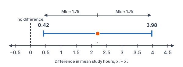
A random sample of 30 students who use a planner study x̄₁ = 12.6 hours a week, with s₁ = 3.2. A separate random sample of 35 students who don’t use one study x̄₂ = 10.4 hours, with s₂ = 3.8. Build a 95% confidence interval for μ₁ − μ₂.
Conditions: two independent random samples, each less than 10% of a large school, and both samples have n ≥ 30.
12.6 - 10.4 = 2.2
Subtract the sample means.
3.2^2 = 10.24
Square s₁.
\dfrac{10.24}{30} \approx 0.3413Divide by n₁.
3.8^2 = 14.44
Square s₂.
\dfrac{14.44}{35} \approx 0.4126Divide by n₂.
0.3413 + 0.4126 = 0.7539
Add the two variances.
\text{SE} = \sqrt{0.7539} \approx 0.8683Take the square root (see square roots).
df = 30 - 1 = 29
Conservative df: the smaller n minus 1.
t^* = \text{invT}(0.975, 29) \approx 2.045Use left area 0.975 with df = 29.
\text{ME} = 2.045 \cdot 0.8683 \approx 1.7757Multiply t* by SE.
2.2 - 1.7757 = 0.4243
Subtract ME from the estimate.
2.2 + 1.7757 = 3.9757
Add ME to the estimate.
Answer: about (0.42, 3.98) hours. We are 95% confident that planner users study between 0.42 and 3.98 more hours a week, on average, than non-users. This is an observational study, so it doesn’t prove the planner causes the extra study time.
Example 2: A small experiment
A gardener randomly assigns 22 seedlings to two groups. The 10 with a new fertilizer grow x̄₁ = 24.5 cm (s₁ = 2.8). The 12 without it grow x̄₂ = 21.0 cm (s₂ = 3.5). Dot plots of both groups show no strong skew or outliers. Build a 90% interval for μ₁ − μ₂.
24.5 - 21.0 = 3.5
Subtract the sample means.
2.8^2 = 7.84
Square s₁.
\dfrac{7.84}{10} = 0.784Divide by n₁.
3.5^2 = 12.25
Square s₂.
\dfrac{12.25}{12} \approx 1.0208Divide by n₂.
0.784 + 1.0208 = 1.8048
Add the two variances.
\text{SE} = \sqrt{1.8048} \approx 1.3434Take the square root.
df = 10 - 1 = 9
Conservative df from the smaller sample.
t^* = \text{invT}(0.95, 9) \approx 1.833For 90%, use left area 0.95.
\text{ME} = 1.833 \cdot 1.3434 \approx 2.4625Multiply t* by SE.
3.5 - 2.4625 = 1.0375
Subtract ME from the estimate.
3.5 + 2.4625 = 5.9625
Add ME to the estimate.
Answer: about (1.04, 5.96) cm. The whole interval is above 0. Because the seedlings were randomly assigned, we can say the fertilizer causes extra growth, between about 1.04 and 5.96 cm on average.
Example 3: An interval that contains 0
A driver times random trips on two routes to work. Route 1: n₁ = 40 trips, x̄₁ = 31.2 minutes, s₁ = 6.5. Route 2: n₂ = 45 trips, x̄₂ = 29.8 minutes, s₂ = 7.1. Build a 99% interval for μ₁ − μ₂.
31.2 - 29.8 = 1.4
Subtract the sample means.
\dfrac{6.5^2}{40} = \dfrac{42.25}{40}Square s₁.
\approx 1.0563
Divide by n₁.
\dfrac{7.1^2}{45} = \dfrac{50.41}{45}Square s₂.
\approx 1.1202
Divide by n₂.
1.0563 + 1.1202 = 2.1765
Add the two variances.
\text{SE} = \sqrt{2.1765} \approx 1.4753Take the square root.
t^* = \text{invT}(0.995, 39) \approx 2.708df = 40 − 1 = 39; left area 0.995 for 99%.
\text{ME} = 2.708 \cdot 1.4753 \approx 3.9951Multiply t* by SE.
1.4 - 3.9951 = -2.5951
Subtract ME from the estimate.
1.4 + 3.9951 = 5.3951
Add ME to the estimate.
Answer: about (−2.60, 5.40) minutes. The interval contains 0, so the data don’t show a convincing difference between the routes. Route 1 could be up to 5.40 minutes slower or up to 2.60 minutes faster.
Example 4: Read calculator output
2-SampTInt gives the 95% interval (−1.8, 6.2) for μ₁ − μ₂. Find the point estimate and the margin of error. Do the data show a difference?
\dfrac{-1.8 + 6.2}{2} = \dfrac{4.4}{2}Add the endpoints.
= 2.2
Divide by 2; the estimate is the midpoint.
\text{ME} = 6.2 - 2.2 = 4Subtract the estimate from the upper endpoint.
Answer: x̄₁ − x̄₂ = 2.2 and ME = 4. The interval contains 0, so the data don’t show a convincing difference.
Example 5: The calculator’s df
Use Example 2 (variances 0.784 and 1.0208, SE ≈ 1.3434). A calculator uses this df formula: df = (v₁ + v₂)² ÷ (v₁²/(n₁ − 1) + v₂²/(n₂ − 1)), where v₁ and v₂ are the two variances. Find this df and the new 90% interval.
1.8048^2 \approx 3.2573
Square the sum of the variances.
0.784^2 \approx 0.6147
Square v₁.
\dfrac{0.6147}{9} \approx 0.0683Divide by n₁ − 1 = 9.
1.0208^2 \approx 1.0420
Square v₂.
\dfrac{1.0420}{11} \approx 0.0947Divide by n₂ − 1 = 11.
0.0683 + 0.0947 = 0.163
Add.
df = \dfrac{3.2573}{0.163} \approx 19.98Divide.
t^* = \text{invT}(0.95, 19.98) \approx 1.725Find t* with the new df.
\text{ME} = 1.725 \cdot 1.3434 \approx 2.3174Multiply t* by SE.
3.5 - 2.3174 = 1.1826
Subtract ME from the estimate.
3.5 + 2.3174 = 5.8174
Add ME to the estimate.
Answer: df ≈ 19.98 and the interval is about (1.18, 5.82) cm. That is a bit narrower than the conservative (1.04, 5.96), because more df gives a smaller t*. Both methods are accepted; the calculator’s is more exact.
Common mistakes
| Mistake | Example of the error | Fix |
|---|---|---|
| Subtracting the variances | √(1.0563 − 1.1202) | Always add the variances under the square root. |
| Forgetting to square s | 3.2/30 + 3.8/35 | Use s₁²/n₁ + s₂²/n₂. |
| Using df = n₁ + n₂ − 1 | df = 64 for samples of 30 and 35 | By hand, use the smaller n minus 1 (df = 29). |
| Using two-sample methods on paired data | Before and after scores for the same 20 students | Use a one-sample t-interval on the differences. |
| Claiming cause from an observational study | “Planners cause more study time” | Only a randomized experiment supports cause and effect. |
Related methods
Paired data
If each value in one group is matched to a value in the other, such as the same person measured twice, the samples are not independent. Find the differences and build a one-sample confidence interval for a mean on them (see matched pairs design).
Testing a difference in means
A two-sample t-test asks whether μ₁ − μ₂ could be 0. An interval that leaves out 0 points the same way as a test that rejects “no difference.”
Practice problems
- Find the conservative df for samples of size 15 and 22.
- Find the SE of x̄₁ − x̄₂ when s₁ = 4, n₁ = 16, s₂ = 6 and n₂ = 25.
- Use Problem 2 with x̄₁ = 50 and x̄₂ = 46. Build a 95% interval for μ₁ − μ₂ with the conservative df.
- A 95% interval for μ₁ − μ₂ is (−3.1, 0.8). Do the data show a difference?
- A 95% interval for μ₁ − μ₂ is (1.2, 4.6) points. Interpret it.
- Twenty students take a quiz before and after a review session. Should you use a two-sample t-interval? Explain.
- 2-SampTInt gives (2.5, 9.1). Find the point estimate and the margin of error.
- An interval for μ₁ − μ₂ is (1.2, 4.6). What is the interval for μ₂ − μ₁?
- Random samples: n₁ = 25, x̄₁ = 78, s₁ = 10 and n₂ = 20, x̄₂ = 72, s₂ = 8. Build a 90% interval for μ₁ − μ₂ with the conservative df.
- A sample of 12 values in one group is strongly skewed with two outliers. Is a two-sample t-interval safe?
Show answers
1.
15 - 1 = 14
Subtract 1 from the smaller sample size.
Answer: df = 14
2.
\dfrac{4^2}{16} = \dfrac{16}{16}Square s₁.
= 1
Divide by n₁.
\dfrac{6^2}{25} = \dfrac{36}{25}Square s₂.
= 1.44
Divide by n₂.
1 + 1.44 = 2.44
Add the variances.
\text{SE} = \sqrt{2.44} \approx 1.562Take the square root.
Answer: SE ≈ 1.562
3.
50 - 46 = 4
Subtract the means.
t^* = \text{invT}(0.975, 15) \approx 2.131df = 16 − 1 = 15.
\text{ME} = 2.131 \cdot 1.562 \approx 3.3286Multiply t* by SE.
4 - 3.3286 = 0.6714
Subtract ME.
4 + 3.3286 = 7.3286
Add ME.
Answer: about (0.67, 7.33)
4.
The interval contains 0.
Answer: No. A difference of 0 is plausible, so there is no convincing difference.
5.
Both endpoints are above 0.
Answer: We are 95% confident that μ₁ is between 1.2 and 4.6 points higher than μ₂.
6.
The same students are measured twice, so the two sets of scores are paired, not independent.
Answer: No. Find each student’s difference and use a one-sample t-interval on the differences.
7.
\dfrac{2.5 + 9.1}{2} = \dfrac{11.6}{2}Add the endpoints.
= 5.8
Divide by 2.
\text{ME} = 9.1 - 5.8 = 3.3Subtract the estimate from the upper endpoint.
Answer: estimate 5.8, ME = 3.3
8.
Switching the order changes every sign, and the endpoints swap places.
Answer: (−4.6, −1.2)
9.
78 - 72 = 6
Subtract the means.
\dfrac{10^2}{25} = \dfrac{100}{25}Square s₁.
= 4
Divide by n₁.
\dfrac{8^2}{20} = \dfrac{64}{20}Square s₂.
= 3.2
Divide by n₂.
4 + 3.2 = 7.2
Add the variances.
\text{SE} = \sqrt{7.2} \approx 2.683Take the square root.
t^* = \text{invT}(0.95, 19) \approx 1.729df = 20 − 1 = 19; left area 0.95.
\text{ME} = 1.729 \cdot 2.683 \approx 4.6389Multiply t* by SE.
6 - 4.6389 = 1.3611
Subtract ME.
6 + 4.6389 = 10.6389
Add ME.
Answer: about (1.36, 10.64)
10.
The sample is small (under 30) and the data are strongly skewed with outliers, so the Normal/Large Sample condition fails for that group.
Answer: No, the interval is not safe for these data.
Confidence interval for a difference in means FAQ
What is the formula for a confidence interval for the difference of two means?
It is (x̄₁ − x̄₂) ± t* √(s₁²/n₁ + s₂²/n₂). The square root is the standard error, and t* comes from a t-distribution.
What degrees of freedom do you use for a two-sample t-interval?
By hand, use the smaller of n₁ − 1 and n₂ − 1, which is a safe, conservative choice. Calculators use a formula that gives a larger, often decimal, df.
Should you pool the variances?
Usually not. The unpooled interval, with Pooled: No on a TI-84, works whether or not the two population standard deviations are equal, so it is the standard choice.
What does it mean if the interval for μ₁ − μ₂ contains 0?
It means the two population means could be equal. The data don’t give convincing evidence of a difference, but they don’t prove the means are the same.
Summary
- The interval is (x̄₁ − x̄₂) ± t* √(s₁²/n₁ + s₂²/n₂).
- By hand, df = the smaller of n₁ − 1 and n₂ − 1; calculators use a larger, exact df.
- Check Random, 10% and Normal/Large Sample for both groups.
- An interval that leaves out 0 shows a real difference; one that contains 0 does not.
- For paired data, use a one-sample t-interval on the differences instead.
Previous lesson: Confidence Interval for a Difference in Proportions
Next lesson: Hypothesis Testing
Back to the Statistics Index