
t-Distribution
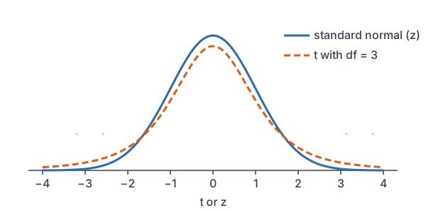
The t-distribution is a bell-shaped curve, centered at 0, with heavier tails than the standard normal curve. You use it instead of z when the population standard deviation σ is unknown and you estimate it with the sample standard deviation s. Its shape depends on the degrees of freedom, df = n − 1.
Before this lesson: Sampling Distribution of a Sample Mean, Standard Normal Distribution and Confidence Intervals
Why we need t instead of z
For a sample mean, the z-score uses σ/√n. But in real studies, σ is almost never known. So you replace σ with s, the sample standard deviation, and get the standard error s/√n.
That swap adds extra uncertainty, because s changes from sample to sample. With a small sample, s can be far from σ. The resulting statistic is no longer exactly normal. It follows a t-distribution, which is more spread out to account for the guesswork in s.
The degrees of freedom tell you which t-curve to use. For one sample, df = n − 1. As df grows, s becomes a better estimate of σ, and the t-curve gets closer to the standard normal curve.
t-distribution formula
t = \dfrac{\bar{x} - \mu}{s / \sqrt{n}} \qquad df = n - 1- Like z, the t statistic counts how many standard errors x̄ is from μ.
- The t-curve is symmetric about 0 and bell-shaped.
- It has heavier tails than z, so t critical values are larger than z critical values.
- As df increases, t critical values get closer to z: at df = ∞, t* = z*.
| df | 90% | 95% | 99% |
|---|---|---|---|
| 5 | 2.015 | 2.571 | 4.032 |
| 10 | 1.812 | 2.228 | 3.169 |
| 20 | 1.725 | 2.086 | 2.845 |
| 30 | 1.697 | 2.042 | 2.750 |
| 60 | 1.671 | 2.000 | 2.660 |
| ∞ (z) | 1.645 | 1.960 | 2.576 |
If your df is not in a printed table, use the next smaller df. That gives a slightly larger t*, which is the safe choice.
Calculator: on a TI-84, invT(left area, df) gives a critical value; for 95%, use invT(0.975, df). tcdf(lower, upper, df) gives an area. In Desmos, use tdist(df).inversecdf(0.975).
t-distribution examples
Example 1: Find df and t*
A random sample of 16 students is used to build a 95% confidence interval for a mean. Find the degrees of freedom and the critical value t*.
df = 16 - 1 = 15
Subtract 1 from n.
1 - 0.95 = 0.05
Find the total tail area.
\dfrac{0.05}{2} = 0.025Split it between the two tails.
t^* = \text{invT}(0.975, 15) \approx 2.131Use left area 0.975 with df = 15.
Answer: df = 15 and t* ≈ 2.131. Compare that with z* = 1.96: the t value is larger.
Example 2: Compute a t statistic
A random sample of 25 batteries has mean life x̄ = 52.4 hours and standard deviation s = 6 hours. The maker claims μ = 50 hours. Find the t statistic and its degrees of freedom.
\sqrt{25} = 5Find √n (see square roots).
\text{SE} = \dfrac{6}{5} = 1.2Divide s by √n.
t = \dfrac{52.4 - 50}{1.2} = \dfrac{2.4}{1.2}Subtract μ from x̄.
= 2.0
Divide.
df = 25 - 1 = 24
Subtract 1 from n.
Answer: t = 2.0 with df = 24. The sample mean is 2 standard errors above the claimed mean.
Example 3: How much wider is t?
For a sample of n = 10, compare the 95% critical values t* and z*. How much wider is a t-interval than a z-interval with the same standard error?
df = 10 - 1 = 9
Find the degrees of freedom.
t^* = \text{invT}(0.975, 9) \approx 2.262Find t*.
\dfrac{2.262}{1.96} \approx 1.154Divide t* by z* = 1.96.
Answer: t* ≈ 2.262, so the t-interval is about 15% wider. With only 10 values, s is a shaky estimate of σ, and the wider interval makes up for it.
Example 4: Find a tail area
Use Example 2. If the true mean is 50 hours, what is the probability of a t statistic of 2.0 or more?
P(t \ge 2.0) = \text{tcdf}(2.0, 10^{99}, 24)Find the area to the right of 2.0 with df = 24.
\approx 0.0285
Read the calculator result.
Answer: about 0.0285. The standard normal curve gives about 0.0228 for z ≥ 2, so the t-curve puts a little more area in the tail.
Example 5: Checking a wait-time claim (word problem)
A coffee shop says customers wait 4 minutes on average. A random sample of 12 customers has x̄ = 4.9 minutes and s = 1.5 minutes. Find the t statistic, and the probability of a t this large or larger if the claim is true.
\sqrt{12} \approx 3.464Find √n.
\text{SE} = \dfrac{1.5}{3.464} \approx 0.4330Divide s by √n.
t = \dfrac{4.9 - 4}{0.4330} = \dfrac{0.9}{0.4330}Subtract μ from x̄.
\approx 2.079
Divide.
df = 12 - 1 = 11
Find the degrees of freedom.
P(t \ge 2.079) \approx 0.031
tcdf(2.079, 10^99, 11).
Answer: t ≈ 2.079 with df = 11, and the probability is about 0.031. A sample mean this high would be fairly unusual if the true mean were 4 minutes. Hypothesis tests later in the course make this reasoning formal.
Common mistakes
| Mistake | Example of the error | Fix |
|---|---|---|
| Using df = n | df = 16 for n = 16 | df = n − 1 = 15. |
| Using z* when σ is unknown | 1.96 for a mean with only s known | Use t* with df = n − 1. |
| Using the wrong left area in invT | invT(0.95, 15) for 95% confidence | Use invT(0.975, 15); half of the 5% goes in each tail. |
| Using σ/√n when only s is known | SE = σ/√n with σ unknown | Use SE = s/√n. |
| Thinking t is a different shape from z | “The t-curve is skewed” | It is symmetric and bell-shaped, just with heavier tails. |
Related methods
t vs. z for proportions
The t-distribution is used for means. For proportions, the standard error comes from p̂ alone, so intervals and tests for proportions still use z (see confidence interval for a proportion).
Margin of error with t
A t-interval has margin of error t^* \cdot s/\sqrt{n}. It works like the margin of error with z, but t* depends on the sample size through df. The next lesson builds the full confidence interval for a mean.
Practice problems
- A sample has n = 40. Find the degrees of freedom.
- Find t* for a 90% confidence interval with df = 12.
- Find t* for a 99% confidence interval with df = 20.
- A sample of 16 has x̄ = 18 and s = 4. Find the t statistic for μ = 20.
- Which is larger: t* for 95% with df = 5, or with df = 30?
- What value does t* for 95% confidence approach as df grows very large?
- A sample of 36 has s = 9. Find the standard error of x̄.
- A sample of 25 has x̄ = 103 and s = 10. Find the t statistic for μ = 100, and its df.
- Use Problem 8. Find P(t \ge 1.5).
- Why does the t-distribution have heavier tails than the standard normal distribution?
Show answers
1.
df = 40 - 1 = 39
Subtract 1 from n.
Answer: 39
2.
1 - 0.90 = 0.10
Find the total tail area.
\dfrac{0.10}{2} = 0.05Split it between the two tails.
t^* = \text{invT}(0.95, 12) \approx 1.782Left area 0.95 with df = 12.
Answer: about 1.782
3.
1 - 0.99 = 0.01
Find the total tail area.
\dfrac{0.01}{2} = 0.005Split it between the two tails.
t^* = \text{invT}(0.995, 20) \approx 2.845Left area 0.995 with df = 20.
Answer: about 2.845
4.
\text{SE} = \dfrac{4}{\sqrt{16}} = \dfrac{4}{4}Divide s by √n, using √16 = 4.
= 1
Divide.
t = \dfrac{18 - 20}{1} = \dfrac{-2}{1}Subtract μ from x̄.
= -2
Divide.
Answer: t = −2 with df = 15
5.
2.571 \gt 2.042
Compare t* for df = 5 and df = 30.
Answer: df = 5 has the larger t*
6.
As df grows, the t-curve approaches the standard normal curve.
Answer: z* = 1.96
7.
\text{SE} = \dfrac{9}{\sqrt{36}} = \dfrac{9}{6}Divide s by √n, using √36 = 6.
= 1.5
Divide.
Answer: 1.5
8.
\text{SE} = \dfrac{10}{\sqrt{25}} = \dfrac{10}{5}Divide s by √n, using √25 = 5.
= 2
Divide.
t = \dfrac{103 - 100}{2} = \dfrac{3}{2}Subtract μ from x̄.
= 1.5
Divide.
df = 25 - 1 = 24
Subtract 1 from n.
Answer: t = 1.5 with df = 24
9.
P(t \ge 1.5) = \text{tcdf}(1.5, 10^{99}, 24) \approx 0.0733Area to the right of 1.5 with df = 24.
Answer: about 0.0733
10.
The standard error uses s, which varies from sample to sample. That extra uncertainty spreads the distribution of t out, especially for small samples.
Answer: because s is an estimate of σ, not the true value
t-distribution FAQ
When do you use a t-distribution instead of z?
Use t for inference about a mean when the population standard deviation σ is unknown and you use the sample standard deviation s instead. In practice, that is almost always.
What are degrees of freedom in a t-distribution?
Degrees of freedom set which t-curve to use. For a one-sample t procedure, df = n − 1. Smaller df means heavier tails and larger critical values.
How do you find a t critical value?
Use a t-table with the right df and confidence level, or invT(left area, df) on a TI-84. For 95% confidence, the left area is 0.975.
Is the t-distribution the same as the normal distribution?
No. Both are symmetric and bell-shaped, but the t-distribution has heavier tails. As df increases, it gets closer and closer to the standard normal distribution.
Summary
- Use t when σ is unknown and the standard error is s/√n.
- The t statistic is t = (\bar{x} - \mu)/(s/\sqrt{n}), with df = n − 1.
- t-curves are symmetric with heavier tails than z, so t* is larger than z*.
- As df grows, t* approaches z*.
- Find t* with a t-table or invT(left area, df).
Previous lesson: Margin of Error
Next lesson: Confidence Interval for a Mean
Back to the Statistics Index