
Hypothesis Testing
Hypothesis testing is a method for using sample data to judge a claim about a population. You state a null hypothesis H₀ (no effect, no change) and an alternative hypothesis Hₐ (what you suspect). Then you ask how surprising the data would be if H₀ were true. Very surprising data count as evidence against H₀.
Before this lesson: Confidence Intervals, Sampling Distribution of a Sample Proportion and Standard Normal Distribution
The logic of a significance test
A hypothesis test works like a trial. The null hypothesis is “innocent until proven guilty.” You assume it is true, then look at the evidence. If the evidence would be very unlikely under H₀, you reject H₀. If not, you fail to reject it.
The null hypothesis H₀ says nothing special is going on: a parameter equals a claimed value. The alternative hypothesis Hₐ is the claim you want evidence for. Both are always about a population parameter, such as p or μ, never about a sample statistic like p̂ or x̄.
A test statistic measures how far the sample result is from the H₀ value, in standard errors. The p-value is the probability of a result at least that extreme if H₀ is true. A small p-value means the data are hard to explain by chance alone.
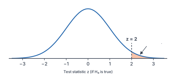
Hypothesis testing formula and steps
\text{test statistic} = \dfrac{\text{statistic} - \text{null value}}{\text{standard error}}- For a proportion: z = \dfrac{\hat{p} - p_0}{\sqrt{p_0(1 - p_0)/n}}, using the null value p₀ in the standard error.
- For a mean: t = \dfrac{\bar{x} - \mu_0}{s/\sqrt{n}}, with df = n − 1 (see t-distribution).
Three forms of the alternative
| Question | Alternative | Type |
|---|---|---|
| Is the parameter greater than the claim? | H_a: p \gt p_0 | One-sided (right tail) |
| Is the parameter less than the claim? | H_a: p \lt p_0 | One-sided (left tail) |
| Is the parameter different from the claim? | H_a: p \ne p_0 | Two-sided (both tails) |
Four steps
- State: write H₀ and Hₐ, define the parameter, and choose the significance level α (often 0.05).
- Plan: name the test and check its conditions.
- Do: compute the test statistic and the p-value.
- Conclude: if p-value ≤ α, reject H₀; if p-value > α, fail to reject H₀. Then answer the question in context.
The significance level α is the cutoff you set before looking at the data. A p-value at or below α is called statistically significant.
Hypothesis testing examples
Example 1: Write hypotheses for a mean
A phone maker claims its battery lasts 10 hours on average. A consumer group suspects the true mean is less. Write the hypotheses.
H_0: \mu = 10
The null states the claim, with an equal sign.
H_a: \mu \lt 10
The alternative states the suspicion.
Answer: H₀: μ = 10 and Hₐ: μ < 10, where μ is the true mean battery life in hours for all phones of this model. This is a one-sided test.
Example 2: Write hypotheses for a proportion
A coin is flipped 200 times to see whether it is fair. Write the hypotheses.
H_0: p = 0.5
A fair coin lands heads half the time.
H_a: p \ne 0.5
“Not fair” could mean too many or too few heads.
Answer: H₀: p = 0.5 and Hₐ: p ≠ 0.5, where p is the true proportion of heads for this coin. This is a two-sided test.
Example 3: Compute a z test statistic
A city says 40% of its high school students walk to school. A random sample of 150 students finds 72 who walk. Find the test statistic for H₀: p = 0.40.
\hat{p} = \dfrac{72}{150} = 0.48Divide walkers by n.
0.40 \cdot 0.60 = 0.24
Multiply p₀(1 − p₀), using the null value.
\dfrac{0.24}{150} = 0.0016Divide by n.
\text{SE} = \sqrt{0.0016} = 0.04Take the square root (see square roots).
0.48 - 0.40 = 0.08
Subtract the null value from p̂.
z = \dfrac{0.08}{0.04} = 2Divide by SE.
Answer: z = 2. The sample proportion is 2 standard errors above the claimed 40%.
Example 4: Make a decision
Use Example 3 with Hₐ: p > 0.40 and α = 0.05. Find the p-value and state a conclusion.
P(Z \ge 2) = \text{normalcdf}(2, 10^{99})Find the area to the right of z = 2 (see normal probability calculations).
\approx 0.0228
Read the calculator result.
0.0228 \lt 0.05
Compare the p-value with α.
Answer: the p-value is about 0.0228, which is less than 0.05, so we reject H₀. There is convincing evidence that more than 40% of the city’s high school students walk to school.
Example 5: Checking a cereal label (word problem)
A cereal box says it holds 500 g. An inspector weighs a random sample of 16 boxes and finds x̄ = 496.5 g and s = 6 g. The weights show no strong skew or outliers. Test H₀: μ = 500 against Hₐ: μ < 500 at α = 0.05.
\sqrt{16} = 4Find √n.
\text{SE} = \dfrac{6}{4} = 1.5Divide s by √n.
496.5 - 500 = -3.5
Subtract the null value from x̄.
t = \dfrac{-3.5}{1.5} \approx -2.333Divide by SE.
df = 16 - 1 = 15
Subtract 1 from n.
P(t \le -2.333) = \text{tcdf}(-10^{99}, -2.333, 15)Find the left-tail area with df = 15.
\approx 0.017
Read the calculator result.
0.017 \lt 0.05
Compare the p-value with α.
Answer: t ≈ −2.333 and the p-value is about 0.017. Since 0.017 < 0.05, reject H₀. There is convincing evidence that the true mean weight of these boxes is less than 500 g.
Common mistakes
| Mistake | Example of the error | Fix |
|---|---|---|
| Writing hypotheses about a statistic | H₀: p̂ = 0.40 | Use the parameter: H₀: p = 0.40. |
| Putting the claim to be proven in H₀ | H₀: μ < 10 | H₀ always has the equal sign; the suspicion goes in Hₐ. |
| Saying “accept H₀” | “We accept that the coin is fair” | Say “fail to reject H₀”; the data just aren’t strong enough. |
| Using p̂ in the standard error of a z-test | SE = √(0.48 · 0.52/150) | Use the null value p₀ in the SE for a test. |
| Choosing Hₐ after seeing the data | Switching to Hₐ: p > 0.40 because p̂ = 0.48 | Write both hypotheses before collecting data. |
Related methods
Tests and confidence intervals
A two-sided test at α = 0.05 matches a 95% confidence interval. If the H₀ value is outside the interval, the test rejects H₀ (see the confidence interval for a mean). An interval also tells you how big the effect might be, which a test alone does not.
What comes next
The next lesson, P-Values, explains how to read and interpret a p-value in detail. Later lessons give the full test for each situation: one proportion, two proportions, one mean, paired data and two means.
Practice problems
- A school claims 80% of its graduates go to college. A reporter thinks the true rate is lower. Write the hypotheses.
- A restaurant says its mean wait time is 12 minutes. A manager wants to know if it is different. Write the hypotheses.
- Is “H₀: x̄ = 50” a correct null hypothesis? Explain.
- For H₀: p = 0.5 with n = 100 and p̂ = 0.56, find the z test statistic.
- For H₀: μ = 20 with n = 25, x̄ = 21.5 and s = 5, find the t test statistic.
- A test gives a p-value of 0.03, and α = 0.05. What is the decision?
- A test gives a p-value of 0.12, and α = 0.05. What is the decision?
- Why do statisticians say “fail to reject H₀” instead of “accept H₀”?
- A drug company asks whether its new drug shortens the mean recovery time from 7 days. Write Hₐ and say whether the test is one-sided or two-sided.
- A test of Hₐ: p < p₀ gives z = −1.8. Find the p-value and the decision at α = 0.05.
Show answers
1.
H_0: p = 0.80
The claim, with an equal sign.
H_a: p \lt 0.80
The reporter’s suspicion.
Answer: H₀: p = 0.80 and Hₐ: p < 0.80, where p is the true proportion of graduates who go to college
2.
H_0: \mu = 12
The claim.
H_a: \mu \ne 12
“Different” means two-sided.
Answer: H₀: μ = 12 and Hₐ: μ ≠ 12
3.
x̄ is a sample statistic. Hypotheses are about the population parameter.
Answer: No. It should be H₀: μ = 50.
4.
0.5 \cdot 0.5 = 0.25
Multiply p₀(1 − p₀).
\dfrac{0.25}{100} = 0.0025Divide by n.
\text{SE} = \sqrt{0.0025} = 0.05Take the square root.
0.56 - 0.5 = 0.06
Subtract p₀ from p̂.
z = \dfrac{0.06}{0.05} = 1.2Divide by SE.
Answer: z = 1.2
5.
\text{SE} = \dfrac{5}{\sqrt{25}} = \dfrac{5}{5}Divide s by √n, using √25 = 5.
= 1
Divide.
21.5 - 20 = 1.5
Subtract μ₀ from x̄.
t = \dfrac{1.5}{1} = 1.5Divide by SE.
Answer: t = 1.5 with df = 24
6.
0.03 \lt 0.05
Compare the p-value with α.
Answer: Reject H₀.
7.
0.12 \gt 0.05
Compare the p-value with α.
Answer: Fail to reject H₀.
8.
Data that fit H₀ don’t prove it. A larger sample might still show a difference.
Answer: Not rejecting H₀ only means the evidence is not strong enough; it doesn’t prove H₀ is true.
9.
“Shortens” points in one direction, below 7.
Answer: Hₐ: μ < 7. It is a one-sided test.
10.
P(Z \le -1.8) = \text{normalcdf}(-10^{99}, -1.8)Find the left-tail area.
\approx 0.0359
Read the calculator result.
0.0359 \lt 0.05
Compare the p-value with α.
Answer: p-value ≈ 0.0359, so reject H₀.
Hypothesis testing FAQ
What is the difference between the null and alternative hypothesis?
The null hypothesis H₀ says there is no effect or no change, and it always contains an equal sign. The alternative Hₐ is what you are looking for evidence of, using <, > or ≠.
What does it mean to reject the null hypothesis?
It means the data would be very unlikely if H₀ were true, since the p-value is at or below α. So you have convincing evidence for Hₐ.
What is a significance level?
The significance level α is the cutoff for “unlikely” that you choose before collecting data. The most common choice is α = 0.05, and 0.01 and 0.10 are also used.
How do you know if a test is one-sided or two-sided?
Look at the question. Words like “more than,” “less than” or “increase” give a one-sided test. Words like “different” or “changed” give a two-sided test.
Summary
- H₀ states that a parameter equals a claimed value; Hₐ states what you suspect (<, > or ≠).
- The test statistic is (statistic − null value) ÷ standard error.
- The p-value is the probability of a result at least this extreme if H₀ is true.
- If p-value ≤ α, reject H₀; otherwise, fail to reject H₀.
- Always state the conclusion in context, about the population parameter.
Previous lesson: Confidence Interval for a Difference in Means
Next lesson: P-Values
Back to the Statistics Index