Type I and Type II Errors: Examples & Power

Type I and Type II errors are the two ways a hypothesis test can be wrong. A Type I error rejects a true null hypothesis H₀. A Type II error fails to reject a false H₀. The chance of a Type I error is α. Power, 1 − β, is the chance a test catches a false H₀.

Before this lesson: Hypothesis Testing, P-Values and One-Proportion z-Test

Two ways a test can be wrong

A test makes a decision from a sample, so it can be fooled by chance. Think of a jury trial. H₀ says the person is innocent. Convicting an innocent person is a Type I error. Letting a guilty person walk away is a Type II error.

Each decision can be right or wrong, depending on the truth, which you never see. The table shows all four cases.

Decision	H₀ is true	H₀ is false
Reject H₀	Type I error (false alarm)	Correct decision (power)
Fail to reject H₀	Correct decision	Type II error (missed effect)

A Type I error is like a false positive: the test says “something is going on” when nothing is. A Type II error is like a false negative: something is going on, but the test misses it.

Type I error, Type II error and power

P(Type I error) = α. If H₀ is true, the test rejects it with probability α, the significance level.
P(Type II error) = β. If H₀ is false, β is the chance the test fails to reject it. β depends on the true value of the parameter.
Power = 1 − β. Power is the chance the test correctly rejects a false H₀.
You only reject when the p-value ≤ α. So after rejecting, only a Type I error is possible. After failing to reject, only a Type II error is possible.

What changes power

A larger sample size n raises power, because the standard error shrinks.
A larger α raises power, but it also raises the Type I error risk.
A true value farther from the null value is easier to detect, so power is higher.
Less variability in the data raises power.

Two normal curves for the sample proportion p̂. The gray curve, centered at 0.50, is the sampling distribution if H₀ is true. The blue curve, centered at 0.55, is the sampling distribution if the true p is 0.55. A dashed cutoff line at p̂ = 0.5411 separates fail to reject (left) from reject H₀ (right). The orange area under the gray curve to the right of the cutoff is α = 0.05. The blue hatched area under the blue curve to the left of the cutoff is β ≈ 0.36. The rest of the blue curve, about 0.64, is the power. — In Example 4, the orange area is the Type I error chance (α = 0.05). The hatched area is the Type II error chance (β ≈ 0.36), and the rest of the blue curve is the power.

Type I and Type II error examples

Example 1: Errors in context (word problem)

A juice machine should fill bottles with 500 mL on average. Each hour, a worker tests H₀: μ = 500 against Hₐ: μ ≠ 500. If the test rejects H₀, the line stops so the machine can be fixed. Describe each error and its cost.

Type I error: the machine is filling correctly (μ = 500), but the test finds convincing evidence that it isn’t. The line stops for no reason, which wastes time and money.
Type II error: the machine is off (μ ≠ 500), but the test doesn’t find convincing evidence. Bottles keep getting the wrong amount, so customers get underfilled bottles or the company gives away extra juice.

Answer: a Type I error is a needless shutdown. A Type II error is a missed problem that keeps going. Always describe errors in the words of the problem, not just “reject a true H₀.”

Example 2: Which error is possible?

A test of H₀: p = 0.30 gives a p-value of 0.03, with α = 0.05. Which type of error could the test have made?

0.03 \lt 0.05

Compare the p-value with α.

The p-value is less than α, so the test rejects H₀. Rejecting can only be wrong if H₀ is true. Answer: only a Type I error is possible. You can’t know whether an error actually happened, because the true p is unknown.

Example 3: The chance of at least one Type I error

A science club runs 20 separate tests, each at α = 0.05. Suppose H₀ is true in every test and the tests are independent. Find the expected number of Type I errors and the chance of at least one.

20 \cdot 0.05 = 1

Multiply the number of tests by α.

1 - 0.05 = 0.95

Find the chance one test makes no error (see the complement rule).

0.95^{20} \approx 0.3585

Multiply for 20 independent tests (see independent events).

1 - 0.3585 = 0.6415

Subtract from 1 to get “at least one.”

Answer: the club should expect about 1 false alarm, and the chance of at least one is about 0.64. This is why a single “significant” result among many tests needs to be checked again with new data.

Example 4: Finding power

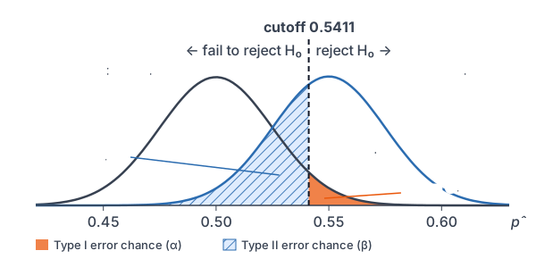
A coach tests H₀: p = 0.50 against Hₐ: p > 0.50 for a player’s free-throw rate, using n = 400 shots and α = 0.05. Suppose the true rate is really p = 0.55. Find the power of the test and β.

First find the cutoff: the smallest p̂ that leads to rejecting H₀.

0.5 \cdot 0.5 = 0.25

Multiply p₀(1 − p₀).

\dfrac{0.25}{400} = 0.000625

Divide by n.

\text{SE}_0 = \sqrt{0.000625} = 0.025

Take the square root (see square roots).

z^* = \text{invNorm}(0.95) \approx 1.645

Find the z that cuts off the top 5%.

1.645 \cdot 0.025 \approx 0.0411

Multiply z* by the standard error.

0.50 + 0.0411 = 0.5411

Add to p₀ to get the cutoff.

The test rejects H₀ when p̂ ≥ 0.5411. Now find the chance of that when p really is 0.55.

0.55 \cdot 0.45 = 0.2475

Multiply p(1 − p) using the true p.

\dfrac{0.2475}{400} = 0.00061875

Divide by n.

\text{SE}_1 = \sqrt{0.00061875} \approx 0.02487

Take the square root.

z = \dfrac{0.5411 - 0.55}{0.02487} = \dfrac{-0.0089}{0.02487}

Subtract the true p from the cutoff.

\approx -0.358

Divide by the standard error.

\text{Power} = \text{normalcdf}(-0.358, 10^{99})

Find the area to the right (see normal probability calculations).

\approx 0.6398

Read the calculator result.

\beta = 1 - 0.6398 = 0.3602

Subtract the power from 1.

Answer: the power is about 0.64 and β ≈ 0.36. If the player really makes 55% of free throws, this test will miss it about 36% of the time.

Example 5: A bigger sample raises power

Repeat Example 4 with n = 900 shots instead of 400. Everything else stays the same.

\dfrac{0.25}{900} \approx 0.0002778

Divide p₀(1 − p₀) = 0.25 by n.

\text{SE}_0 = \sqrt{0.0002778} \approx 0.01667

Take the square root.

1.645 \cdot 0.01667 \approx 0.0274

Multiply z* by the standard error.

0.50 + 0.0274 = 0.5274

Add to p₀ to get the cutoff.

\dfrac{0.2475}{900} = 0.000275

Divide p(1 − p) = 0.2475 by n.

\text{SE}_1 = \sqrt{0.000275} \approx 0.01658

Take the square root.

z = \dfrac{0.5274 - 0.55}{0.01658} = \dfrac{-0.0226}{0.01658}

Subtract the true p from the cutoff.

\approx -1.363

Divide by the standard error.

\text{Power} = \text{normalcdf}(-1.363, 10^{99})

Find the area to the right.

\approx 0.9136

Read the calculator result.

\beta = 1 - 0.9136 = 0.0864

Subtract the power from 1.

Answer: the power rises from about 0.64 to about 0.91, and β drops from 0.36 to about 0.09. The larger sample makes both curves narrower, so they overlap less. α is still 0.05.

Common mistakes

Mistake	Example of the error	Fix
Mixing up the two errors	Calling a false alarm a Type II error	Type I = reject a true H₀ (false alarm). Type II = fail to reject a false H₀ (miss).
Thinking α is the chance H₀ is true	“There is a 5% chance H₀ is true.”	α is the chance of rejecting H₀ if H₀ is true.
Saying an error definitely happened	“We rejected H₀, so we made a Type I error.”	You can only say which error is possible.
Thinking power is 1 − α	“α = 0.05, so power = 0.95.”	Power = 1 − β. It depends on n, α and the true value.
Always choosing a tiny α	Using α = 0.001 to be “safe”	A smaller α lowers the Type I risk but raises β and lowers power.

Related methods

Choosing α from the costs

Pick α by asking which error is worse. If a false alarm is very costly, use a small α such as 0.01. If missing a real effect is worse, a larger α such as 0.10 gives more power.

Planning the sample size

Researchers often choose n before collecting data so the test has power of at least 0.80 for the smallest effect they care about. This is like choosing n for a target margin of error in a confidence interval.

Practice problems

A drug company tests H₀: a new drug works no better than the old one. Describe a Type I error in context.
Use Problem 1. Describe a Type II error in context.
A test uses α = 0.10. If H₀ is true, what is the chance of a Type I error?
A test has power 0.85 against a certain alternative. Find β.
A test gives a p-value of 0.12 with α = 0.05. Which type of error could have happened?
A lab runs 10 independent tests at α = 0.05, and H₀ is true in all of them. Find the chance of at least one Type I error.
Does each change raise or lower power? (a) n goes from 100 to 400. (b) α goes from 0.05 to 0.01.
A smoke detector tests H₀: there is no fire. Which error is a false alarm? Which error is more serious?
A test of H₀: p = 0.40 against Hₐ: p > 0.40 uses n = 600 and α = 0.05. Find the power if the true p is 0.45.
Use Problem 9. Find β, and name two ways to raise the power.

Show answers

Answer: The test concludes the new drug works better when it really doesn’t. Patients may switch to a drug that is no better.

Answer: The new drug really works better, but the test doesn’t find convincing evidence. A better drug may not be used.

Answer: 0.10, because P(Type I error) = α.

\beta = 1 - 0.85 = 0.15

Subtract the power from 1.

Answer: β = 0.15

0.12 \gt 0.05

Compare the p-value with α.

Answer: The test fails to reject H₀, so only a Type II error is possible.

1 - 0.05 = 0.95

Chance one test makes no error.

0.95^{10} \approx 0.5987

Multiply for 10 independent tests.

1 - 0.5987 = 0.4013

Subtract from 1.

Answer: about 0.40

Answer: (a) Raises power, because a larger n shrinks the standard error. (b) Lowers power, because a smaller α moves the cutoff farther out.

Answer: A false alarm is a Type I error (the alarm sounds with no fire). A Type II error (no alarm during a real fire) is more serious, so detectors are set to be very sensitive.

0.4 \cdot 0.6 = 0.24

Multiply p₀(1 − p₀).

\dfrac{0.24}{600} = 0.0004

Divide by n.

\text{SE}_0 = \sqrt{0.0004} = 0.02

Take the square root.

1.645 \cdot 0.02 = 0.0329

Multiply z* by the standard error.

0.40 + 0.0329 = 0.4329

Add to p₀ to get the cutoff.

0.45 \cdot 0.55 = 0.2475

Multiply p(1 − p) using the true p.

\dfrac{0.2475}{600} = 0.0004125

Divide by n.

\text{SE}_1 = \sqrt{0.0004125} \approx 0.02031

Take the square root.

z = \dfrac{0.4329 - 0.45}{0.02031} = \dfrac{-0.0171}{0.02031}

Subtract the true p from the cutoff.

\approx -0.842

Divide by the standard error.

\text{Power} = \text{normalcdf}(-0.842, 10^{99}) \approx 0.8001

Find the area to the right.

Answer: power ≈ 0.80

10.

\beta = 1 - 0.8001 = 0.1999

Subtract the power from 1.

Answer: β ≈ 0.20. To raise power, use a larger sample or a larger α (power is also higher when the true p is farther from 0.40).

Type I and Type II errors FAQ

What is the difference between a Type I and a Type II error?

A Type I error rejects a true null hypothesis, like a false alarm. A Type II error fails to reject a false null hypothesis, like missing a real effect.

What is the probability of a Type I error?

It equals the significance level α. If you test at α = 0.05 and H₀ is true, the test wrongly rejects H₀ 5% of the time.

What is the power of a test?

Power is the chance that a test rejects H₀ when H₀ is false. It equals 1 − β, where β is the chance of a Type II error.

How do you increase the power of a test?

Use a larger sample, a larger α, or data with less variability. Power is also higher when the true value is farther from the null value.

Summary

A Type I error rejects a true H₀ (a false alarm). Its probability is α.
A Type II error fails to reject a false H₀ (a miss). Its probability is β.
Power = 1 − β, the chance of correctly rejecting a false H₀.
After rejecting, only a Type I error is possible; after failing to reject, only a Type II error is possible.
Larger n, larger α and a bigger true effect all raise power.

Previous lesson: One-Proportion z-Test

Next lesson: Two-Proportion z-Test

Back to the Statistics Index