
Chi-Square Test for Independence
A chi-square test for independence checks whether two categorical variables are related in a two-way table. Find each cell’s expected count, E = (row total × column total) ÷ table total, then add χ² = Σ (O − E)²/E over all cells. Use df = (rows − 1)(columns − 1). A small p-value is evidence of an association.
Before this lesson: Two-Way Tables, Independent Events and Chi-Square Goodness-of-Fit Test
How the test works
Suppose you ask 200 randomly chosen students their grade group and their favorite school lunch. If grade group and lunch choice are independent, each grade group should have about the same mix of lunch choices.
The expected counts show what the table would look like if H₀ (no association) were true. They keep the same row and column totals as your data. Then χ² measures how far the real counts are from those expected counts, cell by cell.
The same math answers two kinds of questions. A test for independence uses one random sample and two variables. A test for homogeneity uses separate random samples from two or more groups and one variable. It asks whether the groups have the same distribution.
Chi-square test for independence formula
E = \dfrac{(\text{row total})(\text{column total})}{\text{table total}}\chi^2 = \sum \dfrac{(O - E)^2}{E}, \qquad \text{df} = (r - 1)(c - 1)- r is the number of rows and c is the number of columns (not counting totals).
- Independence: H₀: there is no association between the two variables. Hₐ: there is an association.
- Homogeneity: H₀: the distribution of the variable is the same for every group. Hₐ: the distributions are not all the same.
- The p-value is the right tail: χ²cdf(χ², 10^99, df).
- On a TI-84: enter the observed counts in matrix [A] (2nd, x⁻¹, EDIT). Then STAT, TESTS, C:χ²-Test with Observed: [A] and Expected: [B]. The calculator fills [B] with the expected counts.
Conditions
- Random: one random sample (independence), or independent random samples or a randomized experiment (homogeneity).
- 10%: when sampling without replacement, each sample is at most 10% of its population.
- Large Counts: every expected count is at least 5.
Chi-square test for independence examples
Example 1: Find an expected count
In a table of 200 students, the “grades 9–10” row has a total of 100 and the “pizza” column has a total of 85. Find the expected count for that cell.
100 \cdot 85 = 8500
Multiply the row total by the column total.
\dfrac{8500}{200} = 42.5Divide by the table total.
Answer: E = 42.5. If grade group and lunch choice were independent, about 42.5 of the 100 younger students would pick pizza.
Example 2: Lunch choice and grade group (word problem)
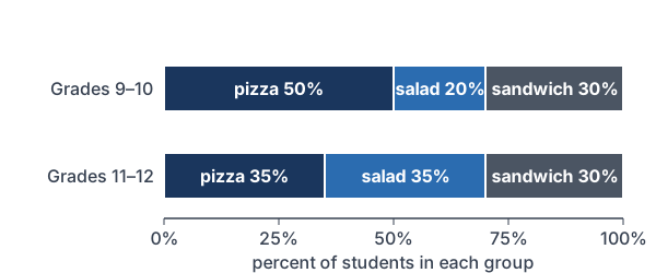
A random sample of 200 students at a large school gives this table. Is there convincing evidence of an association between grade group and lunch choice? Use α = 0.05.
| Group | Pizza | Salad | Sandwich | Total |
|---|---|---|---|---|
| Grades 9–10 | 50 | 20 | 30 | 100 |
| Grades 11–12 | 35 | 35 | 30 | 100 |
| Total | 85 | 55 | 60 | 200 |
State: H₀: there is no association between grade group and lunch choice for students at this school. Hₐ: there is an association. Plan: chi-square test for independence. The sample is random, 200 is less than 10% of the school, and the expected counts below are all at least 5.
\dfrac{100 \cdot 85}{200} = 42.5Expected pizza count for each row (both rows total 100).
\dfrac{100 \cdot 55}{200} = 27.5Expected salad count for each row.
\dfrac{100 \cdot 60}{200} = 30Expected sandwich count for each row.
\dfrac{(50 - 42.5)^2}{42.5} = \dfrac{56.25}{42.5} \approx 1.324Grades 9–10, pizza.
\dfrac{(20 - 27.5)^2}{27.5} = \dfrac{56.25}{27.5} \approx 2.045Grades 9–10, salad.
\dfrac{(30 - 30)^2}{30} = 0Grades 9–10, sandwich.
\dfrac{(35 - 42.5)^2}{42.5} = \dfrac{56.25}{42.5} \approx 1.324Grades 11–12, pizza.
\dfrac{(35 - 27.5)^2}{27.5} = \dfrac{56.25}{27.5} \approx 2.045Grades 11–12, salad.
\dfrac{(30 - 30)^2}{30} = 0Grades 11–12, sandwich.
1.324 + 2.045 + 0 + 1.324 + 2.045 + 0 = 6.738
Add the six terms to get χ².
\text{df} = (2 - 1)(3 - 1) = 2Multiply (rows − 1) by (columns − 1).
P(\chi^2 \ge 6.738) = \chi^2\text{cdf}(6.738, 10^{99}, 2)Find the right-tail area.
\approx 0.0344
Read the calculator result.
0.0344 \lt 0.05
Compare the p-value with α.
Conclude: the p-value is about 0.0344, which is less than 0.05, so reject H₀. There is convincing evidence of an association between grade group and lunch choice. The biggest terms are for salad: older students chose salad more often than expected.
Example 3: A test for homogeneity
A researcher takes separate random samples of 100 students at each of three high schools and asks whether they play a school sport. School A: 48 yes, 52 no. School B: 55 yes, 45 no. School C: 42 yes, 58 no. Is the proportion who play a sport the same at all three schools? Use α = 0.05.
\dfrac{100 \cdot 145}{300} \approx 48.333Expected “yes” count at each school (145 yes in all).
\dfrac{100 \cdot 155}{300} \approx 51.667Expected “no” count at each school (155 no in all).
\dfrac{(48 - 48.333)^2}{48.333} \approx 0.002School A, yes.
\dfrac{(52 - 51.667)^2}{51.667} \approx 0.002School A, no.
\dfrac{(55 - 48.333)^2}{48.333} \approx 0.920School B, yes.
\dfrac{(45 - 51.667)^2}{51.667} \approx 0.860School B, no.
\dfrac{(42 - 48.333)^2}{48.333} \approx 0.830School C, yes.
\dfrac{(58 - 51.667)^2}{51.667} \approx 0.776School C, no.
0.002 + 0.002 + 0.920 + 0.860 + 0.830 + 0.776 = 3.390
Add the six terms to get χ².
\text{df} = (2 - 1)(3 - 1) = 2Multiply (rows − 1) by (columns − 1).
P(\chi^2 \ge 3.390) = \chi^2\text{cdf}(3.390, 10^{99}, 2) \approx 0.184Find the right-tail area.
0.184 \gt 0.05
Compare the p-value with α.
Answer: with H₀: the proportion who play a sport is the same at all three schools, the p-value is about 0.184, so fail to reject H₀. The data don’t give convincing evidence that the proportions differ.
Example 4: Independence or homogeneity?
For each study, name the test and find df. (a) A random sample of 500 adults is asked their age group (4 groups) and main news source (3 choices). (b) Separate random samples from 3 towns are asked their favorite of 5 parks.
(4 - 1)(3 - 1) = 6
df for part (a).
(3 - 1)(5 - 1) = 8
df for part (b).
Answer: (a) Test for independence, with df = 6: one sample, two variables. (b) Test for homogeneity, with df = 8: three separate samples, one variable.
Example 5: Checking Large Counts
A table of 60 people has a row total of 12 and a column total of 15. Is the expected count for that cell large enough?
\dfrac{12 \cdot 15}{60} = \dfrac{180}{60} = 3Find the expected count.
3 \lt 5
Compare with 5.
Answer: No. This expected count is only 3, so the Large Counts condition fails. Collect more data, or combine categories if that makes sense in context.
Common mistakes
| Mistake | Example of the error | Fix |
|---|---|---|
| Using the wrong df | df = 6 − 1 = 5 for a 2 × 3 table | df = (2 − 1)(3 − 1) = 2. |
| Wrong expected count formula | E = 200/6 for every cell | E = (row total × column total) ÷ table total. |
| Including the totals as categories | Counting the “Total” row in r | Count only the data rows and columns. |
| Using percents instead of counts | O = 50% in a cell | Use the counts in the table. |
| Claiming cause from an association | “Being older causes students to pick salad.” | An observational sample shows association, not cause. |
Related methods
Two groups and two outcomes
For a 2 × 2 table, the chi-square test gives the same p-value as a two-sided two-proportion z-test, because χ² = z².
One variable
If you have one categorical variable and a claimed distribution, use the chi-square goodness-of-fit test instead.
Practice problems
- A cell has a row total of 60 and a column total of 50 in a table of 200. Find its expected count.
- Find df for a table with 4 rows and 3 columns.
- A test gives χ² = 8.4 with df = 3. Find the p-value.
- A cell has O = 30 and E = 24. Find its term (O − E)²/E.
- Independence or homogeneity? (a) A random sample of 500 adults is asked their age group and main news source. (b) Random samples from 3 schools are asked their favorite subject.
- A random sample of 120 adults is classified by exercise (yes or no) and sleep quality (good or poor). Exercise: 40 good, 20 poor. No exercise: 25 good, 35 poor. Test for an association at α = 0.05.
- Write H₀ and Hₐ for part (a) of Problem 5.
- A test for homogeneity of favorite music genre across three grades gives a p-value of 0.41 with α = 0.05. Write the conclusion.
- The smallest expected count in a table is 4.2. Is the Large Counts condition met?
- Use Problem 6. Does the result show that exercise causes better sleep?
Show answers
1.
60 \cdot 50 = 3000
Multiply the row total by the column total.
\dfrac{3000}{200} = 15Divide by the table total.
Answer: E = 15
2.
(4 - 1)(3 - 1) = 3 \cdot 2 = 6
Multiply (rows − 1) by (columns − 1).
Answer: df = 6
3.
P(\chi^2 \ge 8.4) = \chi^2\text{cdf}(8.4, 10^{99}, 3) \approx 0.0384Find the right-tail area.
Answer: about 0.0384
4.
30 - 24 = 6
Subtract E from O.
6^2 = 36
Square the gap.
\dfrac{36}{24} = 1.5Divide by E.
Answer: 1.5
5.
Answer: (a) Independence: one sample, two variables. (b) Homogeneity: separate samples from 3 groups, one variable.
6.
40 + 25 = 65
Column total for good sleep.
20 + 35 = 55
Column total for poor sleep.
\dfrac{60 \cdot 65}{120} = 32.5Expected “good” count in each row (both rows total 60).
\dfrac{60 \cdot 55}{120} = 27.5Expected “poor” count in each row.
\dfrac{(40 - 32.5)^2}{32.5} = \dfrac{56.25}{32.5} \approx 1.731Exercise, good.
\dfrac{(20 - 27.5)^2}{27.5} = \dfrac{56.25}{27.5} \approx 2.045Exercise, poor.
\dfrac{(25 - 32.5)^2}{32.5} = \dfrac{56.25}{32.5} \approx 1.731No exercise, good.
\dfrac{(35 - 27.5)^2}{27.5} = \dfrac{56.25}{27.5} \approx 2.045No exercise, poor.
1.731 + 2.045 + 1.731 + 2.045 = 7.552
Add the terms to get χ².
\text{df} = (2 - 1)(2 - 1) = 1Multiply (rows − 1) by (columns − 1).
P(\chi^2 \ge 7.552) = \chi^2\text{cdf}(7.552, 10^{99}, 1) \approx 0.0060Find the right-tail area.
0.0060 \lt 0.05
Compare with α.
Answer: p-value ≈ 0.006, so reject H₀. There is convincing evidence of an association between exercise and sleep quality.
7.
Answer: H₀: there is no association between age group and main news source among adults. Hₐ: there is an association.
8.
0.41 \gt 0.05
Compare the p-value with α.
Answer: Fail to reject H₀. The data don’t give convincing evidence that the distribution of favorite genre differs across the three grades.
9.
4.2 \lt 5
Compare with 5.
Answer: No. Every expected count must be at least 5.
10.
Answer: No. The data come from an observational sample, so they show an association but not cause and effect. Other factors, such as stress, could affect both.
Chi-square test for independence FAQ
How do you calculate expected counts in a two-way table?
Multiply the cell’s row total by its column total, then divide by the table total. The expected counts keep the same totals as the data.
What are the degrees of freedom for a chi-square test for independence?
df = (number of rows − 1)(number of columns − 1), counting only the data rows and columns. A 2 × 3 table has df = 2.
What is the difference between a test for independence and a test for homogeneity?
A test for independence uses one sample and asks whether two variables are related. A test for homogeneity uses separate samples from several groups and asks whether one variable has the same distribution in each group. The calculations are the same.
How do you do a χ²-Test on a TI-84?
Enter the observed counts in matrix [A]. Press STAT, choose TESTS, then C:χ²-Test, with Observed: [A] and Expected: [B]. Choose Calculate; the expected counts are stored in [B].
Summary
- Use a chi-square test for independence (one sample, two variables) or homogeneity (several samples, one variable) on a two-way table.
- E = (row total × column total) ÷ table total.
- χ² = Σ (O − E)²/E over all cells, with df = (r − 1)(c − 1).
- Check Random, 10% and Large Counts (every expected count at least 5).
- The p-value is the right tail. Look at the largest terms to describe the association.
Previous lesson: Chi-Square Goodness-of-Fit Test
Next lesson: Inference for Regression Slope
Back to the Statistics Index