
Paired t-Test
A paired t-test checks whether the mean difference in matched pairs data is zero. You find each pair’s difference d, then run a one-sample t-test on the differences: t = (x̄_d − 0) ÷ (s_d/√n), with n − 1 degrees of freedom, where n is the number of pairs. A small p-value is evidence of a real mean difference.
Before this lesson: One-Sample t-Test and Block Designs and Matched Pairs
When data are paired
Data are paired when each value in one group is linked to one value in the other. Common examples are before-and-after scores for the same people, twins, or two treatments tried on the same subject.
Pairing removes a lot of the person-to-person variation. A strong student and a weak student may both improve by 4 points. Their raw scores are far apart, but their differences are close. Working with the differences lets the test see the effect clearly.
So a paired t-test is really a one-sample t-test on one list: the differences. The null hypothesis says the true mean difference μ_d is 0.
Paired t-test formula
d = \text{after} - \text{before}, \qquad t = \dfrac{\bar{x}_d - 0}{s_d / \sqrt{n}}, \quad \text{df} = n - 1- x̄_d is the mean of the differences, s_d is their standard deviation, and n is the number of pairs.
- H₀: μ_d = 0. Hₐ is μ_d > 0, μ_d < 0 or μ_d ≠ 0. Say which way you subtracted.
- On a TI-84: put the differences in a list (for example L3 = L2 − L1), then STAT, TESTS, 2:T-Test with μ₀ = 0 on that list.
Conditions
- Random: the pairs come from a random sample, or the treatment order is randomly assigned within each pair.
- 10%: when sampling without replacement, n is at most 10% of the population of pairs.
- Normal/Large Sample: the population of differences is roughly normal, or n ≥ 30. For a small n, graph the differences and check for strong skew or outliers.
Paired t-test examples
Example 1: Find the differences
Four students took a quiz before and after a review game. Before: 6, 8, 5, 7. After: 8, 9, 5, 10. Find each difference (after − before) and the mean difference.
8 - 6 = 2
Subtract for student 1.
9 - 8 = 1
Subtract for student 2.
5 - 5 = 0
Subtract for student 3.
10 - 7 = 3
Subtract for student 4.
2 + 1 + 0 + 3 = 6
Add the differences.
\bar{x}_d = \dfrac{6}{4} = 1.5Divide by the number of pairs.
Answer: the differences are 2, 1, 0 and 3, and the mean difference is 1.5 points.
Example 2: Tutoring scores (word problem)
A tutor randomly selects 8 of her students and records their test scores before and after a month of tutoring. Did scores go up on average? Use α = 0.05.
| Student | 1 | 2 | 3 | 4 | 5 | 6 | 7 | 8 |
|---|---|---|---|---|---|---|---|---|
| Before | 72 | 65 | 80 | 58 | 90 | 77 | 69 | 84 |
| After | 78 | 70 | 79 | 66 | 93 | 82 | 71 | 88 |
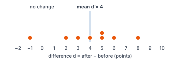
| d = after − before | 6 | 5 | −1 | 8 | 3 | 5 | 2 | 4 |
State: H₀: μ_d = 0 and Hₐ: μ_d > 0, where μ_d is the true mean improvement (after − before). Plan: paired t-test. The students are a random sample, and a dot plot of the 8 differences shows no strong skew or outliers.
6 + 5 + (-1) + 8 + 3 + 5 + 2 + 4 = 32
Add the differences.
\bar{x}_d = \dfrac{32}{8} = 4Divide by the number of pairs.
4 + 1 + 25 + 16 + 1 + 1 + 4 + 0 = 52
Add the squared deviations from 4.
\dfrac{52}{7} \approx 7.429Divide by n − 1 (see standard deviation).
s_d = \sqrt{7.429} \approx 2.726Take the square root (see square roots).
\text{SE} = \dfrac{2.726}{\sqrt{8}} \approx 0.9638Divide s_d by √n.
t = \dfrac{4 - 0}{0.9638} \approx 4.150Divide the mean difference by SE.
\text{df} = 8 - 1 = 7Subtract 1 from the number of pairs.
P(t \ge 4.150) = \text{tcdf}(4.150, 10^{99}, 7)Find the right-tail area.
\approx 0.0021
Read the calculator result.
0.0021 \lt 0.05
Compare the p-value with α.
Conclude: the p-value is about 0.0021, which is less than 0.05, so reject H₀. There is convincing evidence that scores improve on average after a month of tutoring. (Without a control group, we can’t be sure the tutoring caused the gain.)
Example 3: A two-sided test
A company puts Brand A tires on one front wheel and Brand B on the other of 12 randomly chosen cars, flipping a coin for the side. After a year, the differences in tread wear (A − B) have x̄_d = 0.3 mm and s_d = 0.5 mm, with no outliers. Is there a difference? Use α = 0.05.
\sqrt{12} \approx 3.464Take the square root of the number of pairs.
\text{SE} = \dfrac{0.5}{3.464} \approx 0.1443Divide s_d by √n.
t = \dfrac{0.3}{0.1443} \approx 2.079Divide the mean difference by SE.
\text{df} = 12 - 1 = 11Subtract 1 from the number of pairs.
P(t \ge 2.079) = \text{tcdf}(2.079, 10^{99}, 11) \approx 0.0309Find one tail.
2 \cdot 0.0309 = 0.0618
Double it for a two-sided test.
0.0618 \gt 0.05
Compare the p-value with α.
Answer: with H₀: μ_d = 0 and Hₐ: μ_d ≠ 0, the p-value is about 0.0618, so fail to reject H₀. The data don’t give convincing evidence that the brands wear differently.
Example 4: Paired or two samples?
Decide whether each study gives paired data. (a) The heights of 20 sets of twins, one twin from each set eating a new diet. (b) The heights of 20 children on a new diet and 20 different children on a regular diet.
Answer: (a) Paired. Each twin is matched with the other twin, so you analyze the 20 differences with a paired t-test. (b) Not paired. The two groups are separate, so you would use a two-sample t-test.
Example 5: What goes wrong if you ignore the pairing
Suppose someone analyzes the tutoring data in Example 2 as two separate samples. The before scores have x̄ = 74.375 and s ≈ 10.46, and the after scores have x̄ = 78.375 and s ≈ 9.242. Find the two-sample t statistic.
\dfrac{10.46^2}{8} \approx 13.68Square s₁ and divide by n₁.
\dfrac{9.242^2}{8} \approx 10.68Square s₂ and divide by n₂.
13.68 + 10.68 = 24.36
Add the two parts.
\text{SE} = \sqrt{24.36} \approx 4.936Take the square root.
78.375 - 74.375 = 4
Subtract the means.
t = \dfrac{4}{4.936} \approx 0.810Divide by SE.
P(t \ge 0.810) = \text{tcdf}(0.810, 10^{99}, 7) \approx 0.222Find the right-tail area (df = 7, the smaller n − 1).
Answer: t ≈ 0.81 and the p-value is about 0.22, so this wrong analysis finds no evidence of improvement. The standard error is about 4.94 instead of 0.96, because the big differences between students hide the small, steady gains. Always use the paired test when the data are paired.
Common mistakes
| Mistake | Example of the error | Fix |
|---|---|---|
| Using a two-sample test on paired data | Comparing before and after means as separate groups | Find the differences and run a one-sample t-test on them. |
| Using the wrong n | df = 16 − 2 = 14 for 8 students | n is the number of pairs: df = 8 − 1 = 7. |
| Subtracting in different orders | Some d = after − before, some d = before − after | Pick one order, use it for every pair and state it in Hₐ. |
| Checking normality on the raw data | Graphing the before and after scores | Graph the differences; they are what the test uses. |
| Claiming cause without a control group | “Tutoring caused the 4-point gain.” | Before-and-after data alone can’t rule out other causes. |
Related methods
Confidence interval for the mean difference
To estimate the size of the mean difference, build a one-sample t-interval on the differences: x̄_d ± t* · s_d/√n. This is a confidence interval for a mean applied to the list of differences.
Matched pairs experiments
Pairing is planned in a matched pairs design, where each subject gets both treatments in random order or similar subjects are paired. See block designs and matched pairs for how these studies are set up.
Practice problems
- Before: 10, 12, 9, 15. After: 13, 12, 11, 14. Find the differences (after − before) and their mean.
- Use Problem 1. Find s_d.
- Use Problems 1 and 2. Find t and df for H₀: μ_d = 0.
- A study measures each person’s reaction time with and without music. Write H₀ and Hₐ to test whether music slows reaction time (d = with − without).
- Is each study paired? (a) Grip strength of the left and right hand of 25 people. (b) Grip strength of 25 men and 25 women.
- For 20 pairs, x̄_d = −1.5 and s_d = 2.8 (d = new − old). Test Hₐ: μ_d < 0 at α = 0.05.
- A two-sided paired t-test gives t = 1.9 with df = 14. Find the p-value.
- A paired t-test of a new running shoe gives a p-value of 0.27 with α = 0.05. Write the conclusion.
- Why is a paired design often better than two separate groups?
- A paired study has 9 differences, and one difference is far larger than the others. Is a paired t-test safe?
Show answers
1.
13 - 10 = 3
Subtract for pair 1.
12 - 12 = 0
Subtract for pair 2.
11 - 9 = 2
Subtract for pair 3.
14 - 15 = -1
Subtract for pair 4.
3 + 0 + 2 + (-1) = 4
Add the differences.
\bar{x}_d = \dfrac{4}{4} = 1Divide by the number of pairs.
Answer: differences 3, 0, 2, −1; mean x̄_d = 1
2.
4 + 1 + 1 + 4 = 10
Add the squared deviations from 1.
\dfrac{10}{3} \approx 3.333Divide by n − 1.
s_d = \sqrt{3.333} \approx 1.826Take the square root.
Answer: s_d ≈ 1.826
3.
\text{SE} = \dfrac{1.826}{\sqrt{4}} = 0.913Divide s_d by √n.
t = \dfrac{1}{0.913} \approx 1.095Divide the mean difference by SE.
\text{df} = 4 - 1 = 3Subtract 1 from the number of pairs.
Answer: t ≈ 1.095 with df = 3
4.
Answer: H₀: μ_d = 0 and Hₐ: μ_d > 0, where μ_d is the true mean of (with music − without music) reaction times.
5.
Answer: (a) Paired, because each person gives both measurements. (b) Not paired, because the two groups are different people.
6.
\sqrt{20} \approx 4.472Take the square root of the number of pairs.
\text{SE} = \dfrac{2.8}{4.472} \approx 0.6261Divide s_d by √n.
t = \dfrac{-1.5}{0.6261} \approx -2.396Divide the mean difference by SE.
\text{df} = 20 - 1 = 19Subtract 1.
P(t \le -2.396) = \text{tcdf}(-10^{99}, -2.396, 19) \approx 0.0135Find the left-tail area.
0.0135 \lt 0.05
Compare with α.
Answer: p-value ≈ 0.0135, so reject H₀. There is convincing evidence that the mean difference (new − old) is less than 0.
7.
P(t \ge 1.9) = \text{tcdf}(1.9, 10^{99}, 14) \approx 0.0391Find one tail.
2 \cdot 0.0391 = 0.0782
Double it for a two-sided test.
Answer: p-value ≈ 0.0782
8.
0.27 \gt 0.05
Compare the p-value with α.
Answer: Fail to reject H₀. The data don’t give convincing evidence that the new shoe changes the mean result.
9.
Answer: Each pair shares many traits, so the differences vary much less than the raw values. A smaller standard error makes it easier to detect a real effect.
10.
9 \lt 30
Compare the number of pairs with 30.
Answer: No. With only 9 pairs and an outlier in the differences, the Normal/Large Sample condition fails.
Paired t-test FAQ
What is a paired t-test used for?
It tests whether the mean difference between two linked measurements is zero, such as before-and-after scores for the same people or two treatments on the same subjects.
What is the formula for a paired t-test?
Find the difference for each pair. Then t = x̄_d ÷ (s_d/√n), with df = n − 1, where n is the number of pairs.
What is the difference between a paired t-test and a two-sample t-test?
A paired t-test uses one list of differences from linked pairs. A two-sample t-test compares two independent groups that have no natural pairing.
How do you do a paired t-test on a TI-84?
Enter the before values in L1 and the after values in L2, then set L3 = L2 − L1. Choose STAT, TESTS, 2:T-Test, pick Data, set μ₀ = 0 and List: L3, choose the direction of Hₐ and press Calculate.
Summary
- Use a paired t-test when each value in one group is linked to one value in the other.
- Find the differences d, using the same order for every pair.
- t = x̄_d ÷ (s_d/√n), with df = n − 1, where n is the number of pairs.
- Check Random, 10% and Normal/Large Sample on the differences.
- Don’t use a two-sample test on paired data; it hides the effect.
Previous lesson: One-Sample t-Test
Next lesson: Two-Sample t-Test
Back to the Statistics Index