Elementary Matrices: Examples and Inverses

An elementary matrix is the matrix you get by doing one row operation to an identity matrix. Multiplying a matrix A on the left by an elementary matrix E does that same row operation to A, so EA is the result. Every elementary matrix is invertible, and its inverse undoes the row operation.

Before this lesson: Matrix Multiplication, Inverse Matrices and Gaussian Elimination

What an elementary matrix does

Row reduction uses three kinds of row operations: swap two rows, multiply a row by a nonzero number, and add a multiple of one row to another row. Each one can be done by a matrix multiplication instead of by hand.

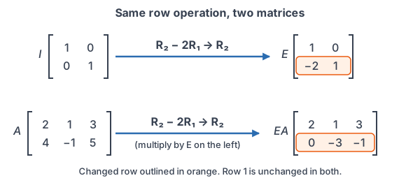
To build the matrix, do the row operation to the identity matrix I. The result is the elementary matrix E. Then, for any matrix A with the right number of rows, the product EA is exactly A with that row operation done to it. This turns row reduction into algebra: a whole chain of row operations becomes a product of matrices.

Top row: the 2 by 2 identity matrix with rows (1, 0) and (0, 1) becomes E with rows (1, 0) and (−2, 1) after the row operation R2 − 2R1. Bottom row: the matrix A with rows (2, 1, 3) and (4, −1, 5) becomes EA with rows (2, 1, 3) and (0, −3, −1). The same row operation label sits on both arrows. — Do a row operation to I to get E. Multiplying by E on the left then does the same row operation to any A.

The three types of elementary matrices

Here Rᵢ means row i, and k is a nonzero number. Each inverse is the elementary matrix for the row operation that undoes the original one.

Row operation	Example (3 × 3)	Inverse
Swap two rows, Rᵢ ↔ Rⱼ	$R_1 \leftrightarrow R_2:\ \begin{bmatrix} 0 & 1 & 0 \\ 1 & 0 & 0 \\ 0 & 0 & 1 \end{bmatrix}$	Swap the same rows again: the matrix is its own inverse.
Scale a row, kRᵢ → Rᵢ	$5R_2 \to R_2:\ \begin{bmatrix} 1 & 0 & 0 \\ 0 & 5 & 0 \\ 0 & 0 & 1 \end{bmatrix}$	Scale by 1/k: here put $\tfrac{1}{5}$ in place of 5.
Add a multiple of a row, Rᵢ + kRⱼ → Rᵢ	$R_3 - 4R_1 \to R_3:\ \begin{bmatrix} 1 & 0 & 0 \\ 0 & 1 & 0 \\ -4 & 0 & 1 \end{bmatrix}$	Add −k times the row instead: here put 4 in place of −4.

Because every elementary matrix has an inverse, every row operation can be reversed. That is why row operations never change the solution set of a system.

Why the [A | I] method works

Suppose row operations with elementary matrices E₁, E₂, …, Eₖ (in that order) reduce a square matrix A to I. Each new operation multiplies on the left, so

E_k \cdots E_2 E_1 A = I \quad\Longrightarrow\quad A^{-1} = E_k \cdots E_2 E_1

When you row reduce the augmented matrix [A | I], the same operations act on both halves. The left half becomes Eₖ⋯E₁A = I, and the right half becomes Eₖ⋯E₁I = A⁻¹. So the right half ends up holding the inverse, as the inverse matrices lesson shows by example.

Solving the same equation for A gives a second fact: every invertible matrix is a product of elementary matrices, namely A = E₁⁻¹E₂⁻¹⋯Eₖ⁻¹. Notice that the order reverses, just as it does for the inverse of any product.

How to use elementary matrices

To find E for a row operation, do that operation to the identity matrix of the right size (m × m when A has m rows).
To do the row operation to A, multiply on the left: EA.
To undo it, use E⁻¹, the elementary matrix of the reverse operation.
To combine several operations, multiply their matrices with the latest operation on the left: E₂E₁ means “first E₁, then E₂.”
To find A⁻¹, reduce A to I, record each Eᵢ and multiply them in reverse order of use.

Elementary matrices examples

Example 1: Name the row operation and find the inverse

Which row operation does E = [1 0 0; 0 1 0; −3 0 1] perform? Find E⁻¹ and check that EE⁻¹ = I. (Rows are separated by semicolons.)

E = \begin{bmatrix} 1 & 0 & 0 \\ 0 & 1 & 0 \\ -3 & 0 & 1 \end{bmatrix}

E differs from I only in row 3, column 1.

R_3 - 3R_1 \to R_3

Row 3 of E is row 3 of I plus −3 times row 1 of I.

R_3 + 3R_1 \to R_3

The reverse operation adds 3 times row 1 back.

E^{-1} = \begin{bmatrix} 1 & 0 & 0 \\ 0 & 1 & 0 \\ 3 & 0 & 1 \end{bmatrix}

Do the reverse operation to I.

EE^{-1} = \begin{bmatrix} 1 & 0 & 0 \\ 0 & 1 & 0 \\ -3(1) + 1(3) & 0 & 1 \end{bmatrix}

Only entry (3, 1) needs work: row 3 of E times column 1 of E⁻¹.

= \begin{bmatrix} 1 & 0 & 0 \\ 0 & 1 & 0 \\ 0 & 0 & 1 \end{bmatrix}

−3 + 3 = 0, so the product is I.

Answer: E does R₃ − 3R₁ → R₃, and E⁻¹ = [1 0 0; 0 1 0; 3 0 1].

Example 2: Do a row operation by multiplying

Let A = [2 1 3; 4 −1 5]. Find the elementary matrix E for R₂ − 2R₁ → R₂, then compute EA.

E = \begin{bmatrix} 1 & 0 \\ -2 & 1 \end{bmatrix}

A has 2 rows, so do R₂ − 2R₁ to the 2 × 2 identity.

EA = \begin{bmatrix} 1(2) + 0(4) & 1(1) + 0(-1) & 1(3) + 0(5) \\ -2(2) + 1(4) & -2(1) + 1(-1) & -2(3) + 1(5) \end{bmatrix}

Multiply rows of E by columns of A (see matrix multiplication).

= \begin{bmatrix} 2 & 1 & 3 \\ 0 & -3 & -1 \end{bmatrix}

Multiply and add in each entry.

Answer: EA = [2 1 3; 0 −3 −1]. Row 1 is unchanged and row 2 became R₂ − 2R₁, just as the row operation does by hand.

Example 3: Find an inverse from elementary matrices

Let A = [1 2; 3 7]. Reduce A to I, write the elementary matrix for each step, and use them to find A⁻¹.

\begin{bmatrix} 1 & 2 \\ 3 & 7 \end{bmatrix} \to \begin{bmatrix} 1 & 2 \\ 0 & 1 \end{bmatrix}

R₂ − 3R₁ → R₂. Row 2: (3 − 3, 7 − 6) = (0, 1).

E_1 = \begin{bmatrix} 1 & 0 \\ -3 & 1 \end{bmatrix}

Do R₂ − 3R₁ to I.

\begin{bmatrix} 1 & 2 \\ 0 & 1 \end{bmatrix} \to \begin{bmatrix} 1 & 0 \\ 0 & 1 \end{bmatrix}

R₁ − 2R₂ → R₁. Row 1: (1 − 0, 2 − 2) = (1, 0).

E_2 = \begin{bmatrix} 1 & -2 \\ 0 & 1 \end{bmatrix}

Do R₁ − 2R₂ to I.

A^{-1} = E_2E_1

The later operation goes on the left.

= \begin{bmatrix} 1(1) + (-2)(-3) & 1(0) + (-2)(1) \\ 0(1) + 1(-3) & 0(0) + 1(1) \end{bmatrix}

Multiply E₂ by E₁.

= \begin{bmatrix} 7 & -2 \\ -3 & 1 \end{bmatrix}

Multiply and add in each entry.

Answer: A⁻¹ = [7 −2; −3 1]. Check: the 2 × 2 formula gives (1/1)[7 −2; −3 1], since det A = 7 − 6 = 1.

Example 4: Write a matrix as a product of elementary matrices

Write A = [2 6; 1 4] as a product of elementary matrices.

\begin{bmatrix} 2 & 6 \\ 1 & 4 \end{bmatrix} \to \begin{bmatrix} 1 & 3 \\ 1 & 4 \end{bmatrix},\; E_1 = \begin{bmatrix} \tfrac{1}{2} & 0 \\ 0 & 1 \end{bmatrix}

½R₁ → R₁. Row 1: (2/2, 6/2) = (1, 3).

\begin{bmatrix} 1 & 3 \\ 1 & 4 \end{bmatrix} \to \begin{bmatrix} 1 & 3 \\ 0 & 1 \end{bmatrix},\; E_2 = \begin{bmatrix} 1 & 0 \\ -1 & 1 \end{bmatrix}

R₂ − R₁ → R₂. Row 2: (1 − 1, 4 − 3) = (0, 1).

\begin{bmatrix} 1 & 3 \\ 0 & 1 \end{bmatrix} \to \begin{bmatrix} 1 & 0 \\ 0 & 1 \end{bmatrix},\; E_3 = \begin{bmatrix} 1 & -3 \\ 0 & 1 \end{bmatrix}

R₁ − 3R₂ → R₁. Row 1: (1 − 0, 3 − 3) = (1, 0).

A = E_1^{-1}E_2^{-1}E_3^{-1}

Solve E₃E₂E₁A = I for A; the order reverses.

A = \begin{bmatrix} 2 & 0 \\ 0 & 1 \end{bmatrix}\begin{bmatrix} 1 & 0 \\ 1 & 1 \end{bmatrix}\begin{bmatrix} 1 & 3 \\ 0 & 1 \end{bmatrix}

Invert each one: 2R₁, then R₂ + R₁, then R₁ + 3R₂.

\begin{bmatrix} 2 & 0 \\ 0 & 1 \end{bmatrix}\begin{bmatrix} 1 & 0 \\ 1 & 1 \end{bmatrix} = \begin{bmatrix} 2 & 0 \\ 1 & 1 \end{bmatrix}

Check: multiply the first two factors.

\begin{bmatrix} 2 & 0 \\ 1 & 1 \end{bmatrix}\begin{bmatrix} 1 & 3 \\ 0 & 1 \end{bmatrix} = \begin{bmatrix} 2 & 6 \\ 1 & 4 \end{bmatrix}

Multiply by the third factor: the result is A.

Answer: A = [2 0; 0 1][1 0; 1 1][1 3; 0 1].

Example 5: One matrix for a weekly table edit

A café records its weekend orders in Q = [120 150; 40 35; 60 80]. The rows are coffee, tea and pastry plates, and the columns are Saturday and Sunday. Each week the owner (1) doubles row 3, because every plate holds two pastries, and then (2) adds the tea row to the coffee row, so row 1 counts all hot drinks. Find one matrix M that does both edits, and apply it to Q.

E_1 = \begin{bmatrix} 1 & 0 & 0 \\ 0 & 1 & 0 \\ 0 & 0 & 2 \end{bmatrix}

Edit 1 is 2R₃ → R₃. Q has 3 rows, so start from the 3 × 3 identity.

E_2 = \begin{bmatrix} 1 & 1 & 0 \\ 0 & 1 & 0 \\ 0 & 0 & 1 \end{bmatrix}

Edit 2 is R₁ + R₂ → R₁.

M = E_2E_1 = \begin{bmatrix} 1 & 1 & 0 \\ 0 & 1 & 0 \\ 0 & 0 & 1 \end{bmatrix}\begin{bmatrix} 1 & 0 & 0 \\ 0 & 1 & 0 \\ 0 & 0 & 2 \end{bmatrix}

The later edit goes on the left.

= \begin{bmatrix} 1 & 1 & 0 \\ 0 & 1 & 0 \\ 0 & 0 & 2 \end{bmatrix}

Multiply: E₁ on the right doubles column 3 of E₂.

MQ = \begin{bmatrix} 120 + 40 & 150 + 35 \\ 40 & 35 \\ 2(60) & 2(80) \end{bmatrix}

Row 1 of M adds rows 1 and 2 of Q; row 3 doubles row 3.

= \begin{bmatrix} 160 & 185 \\ 40 & 35 \\ 120 & 160 \end{bmatrix}

Add and multiply.

Answer: M = [1 1 0; 0 1 0; 0 0 2], and MQ = [160 185; 40 35; 120 160]: 160 hot drinks and 120 pastries on Saturday, 185 hot drinks and 160 pastries on Sunday. Next week the owner can just compute M times the new table.

Common mistakes

Mistake	Example of the error	Fix
Multiplying on the right	Computing AE to do R₂ − 2R₁ on A	EA does a row operation. AE does a column operation instead.
Putting the factors in the wrong order	Writing A⁻¹ = E₁E₂ in Example 3	The latest operation goes on the left: A⁻¹ = E₂E₁.
Keeping the sign when inverting	Saying the inverse of R₃ − 3R₁ → R₃ is the same matrix	Undo it: the inverse adds 3R₁, so the −3 becomes 3.
Scaling a row by 0	Calling [1 0; 0 0] elementary because it “scales row 2”	Scaling uses a nonzero k. Multiplying by 0 cannot be undone.
Using the wrong size of I	Using a 3 × 3 matrix for a row operation on a 2 × 3 matrix	E must be m × m, where m is the number of rows of A.

Related ideas

Determinants of elementary matrices. A row swap matrix has determinant −1, a scaling matrix has determinant k, and a row-replacement matrix has determinant 1. These values, together with det(EA) = det E · det A, explain how row operations change a determinant of a matrix. Properties of Determinants uses this.

Linking to other lessons. Each elementary matrix is the standard matrix of a linear transformation, so a product of them is a composition of linear transformations. The Invertible Matrix Theorem adds “A is a product of elementary matrices” to its list, and LU Decomposition records the row-replacement matrices from Gaussian elimination to factor A.

Practice problems

Write the 3 × 3 elementary matrix for R₂ ↔ R₃.
Write the 3 × 3 elementary matrix E for R₃ + 4R₁ → R₃, and find E⁻¹.
Which row operation does E = [1 0; 0 −6] perform? Find E⁻¹.
E = [0 1; 1 0] and A = [3 −2; 5 1]. Compute EA.
E = [1 0 0; 0 1 0; 0 2 1] and A = [1 0 2; 3 −1 4; 0 1 −3]. Compute EA.
Find the inverse of E = [1 0 0; 0 1 −5; 0 0 1].
A = [1 3; 2 5]. Reduce A to I, record each elementary matrix, and find A⁻¹ as their product.
Write A = [1 0; 4 3] as a product of elementary matrices.
Find one 2 × 2 matrix M that first swaps the two rows and then adds 3 times row 1 to row 2.
Which of these are elementary matrices? (a) [1 0; 3 1] (b) [2 0; 0 3] (c) [0 1; 1 0] (d) [1 0; 0 0]

Show answers

\begin{bmatrix} 1 & 0 & 0 \\ 0 & 0 & 1 \\ 0 & 1 & 0 \end{bmatrix}

Swap rows 2 and 3 of the 3 × 3 identity.

Answer: [1 0 0; 0 0 1; 0 1 0], which is its own inverse.

E = \begin{bmatrix} 1 & 0 & 0 \\ 0 & 1 & 0 \\ 4 & 0 & 1 \end{bmatrix}

Do R₃ + 4R₁ to I: row 3 becomes (0 + 4, 0, 1).

E^{-1} = \begin{bmatrix} 1 & 0 & 0 \\ 0 & 1 & 0 \\ -4 & 0 & 1 \end{bmatrix}

The reverse operation is R₃ − 4R₁ → R₃.

Answer: E = [1 0 0; 0 1 0; 4 0 1] and E⁻¹ = [1 0 0; 0 1 0; −4 0 1].

-6R_2 \to R_2

E is I with row 2 multiplied by −6.

E^{-1} = \begin{bmatrix} 1 & 0 \\ 0 & -\tfrac{1}{6} \end{bmatrix}

Undo it by multiplying row 2 by −1/6.

Answer: E multiplies row 2 by −6; E⁻¹ = [1 0; 0 −1/6].

EA = \begin{bmatrix} 0(3) + 1(5) & 0(-2) + 1(1) \\ 1(3) + 0(5) & 1(-2) + 0(1) \end{bmatrix}

Multiply rows of E by columns of A.

= \begin{bmatrix} 5 & 1 \\ 3 & -2 \end{bmatrix}

Multiply and add.

Answer: EA = [5 1; 3 −2], which is A with its rows swapped.

R_3 + 2R_2 \to R_3

E is I with 2 added in row 3, column 2.

\text{row 3 of } EA = (0 + 2(3),\ 1 + 2(-1),\ -3 + 2(4))

Rows 1 and 2 stay the same; row 3 becomes R₃ + 2R₂.

= (6, -1, 5)

Multiply and add.

EA = \begin{bmatrix} 1 & 0 & 2 \\ 3 & -1 & 4 \\ 6 & -1 & 5 \end{bmatrix}

Write the new matrix.

Answer: EA = [1 0 2; 3 −1 4; 6 −1 5].

R_2 - 5R_3 \to R_2

E is I with −5 in row 2, column 3.

E^{-1} = \begin{bmatrix} 1 & 0 & 0 \\ 0 & 1 & 5 \\ 0 & 0 & 1 \end{bmatrix}

The reverse is R₂ + 5R₃ → R₂.

Answer: E⁻¹ = [1 0 0; 0 1 5; 0 0 1].

\begin{bmatrix} 1 & 3 \\ 2 & 5 \end{bmatrix} \to \begin{bmatrix} 1 & 3 \\ 0 & -1 \end{bmatrix},\; E_1 = \begin{bmatrix} 1 & 0 \\ -2 & 1 \end{bmatrix}

R₂ − 2R₁ → R₂. Row 2: (2 − 2, 5 − 6) = (0, −1).

\begin{bmatrix} 1 & 3 \\ 0 & -1 \end{bmatrix} \to \begin{bmatrix} 1 & 3 \\ 0 & 1 \end{bmatrix},\; E_2 = \begin{bmatrix} 1 & 0 \\ 0 & -1 \end{bmatrix}

−R₂ → R₂. Row 2: (0, 1).

\begin{bmatrix} 1 & 3 \\ 0 & 1 \end{bmatrix} \to \begin{bmatrix} 1 & 0 \\ 0 & 1 \end{bmatrix},\; E_3 = \begin{bmatrix} 1 & -3 \\ 0 & 1 \end{bmatrix}

R₁ − 3R₂ → R₁. Row 1: (1 − 0, 3 − 3) = (1, 0).

E_2E_1 = \begin{bmatrix} 1 & 0 \\ 2 & -1 \end{bmatrix}

Multiply the first two, latest on the left: row 2 is (0 + 2, 0 − 1).

A^{-1} = E_3(E_2E_1) = \begin{bmatrix} 1(1) + (-3)(2) & 1(0) + (-3)(-1) \\ 0(1) + 1(2) & 0(0) + 1(-1) \end{bmatrix}

Multiply by E₃ on the left.

= \begin{bmatrix} -5 & 3 \\ 2 & -1 \end{bmatrix}

Multiply and add.

Answer: A⁻¹ = [−5 3; 2 −1]. Check: det A = 5 − 6 = −1, and (1/−1)[5 −3; −2 1] gives the same matrix.

\begin{bmatrix} 1 & 0 \\ 4 & 3 \end{bmatrix} \to \begin{bmatrix} 1 & 0 \\ 0 & 3 \end{bmatrix},\; E_1 = \begin{bmatrix} 1 & 0 \\ -4 & 1 \end{bmatrix}

R₂ − 4R₁ → R₂. Row 2: (4 − 4, 3 − 0) = (0, 3).

\begin{bmatrix} 1 & 0 \\ 0 & 3 \end{bmatrix} \to \begin{bmatrix} 1 & 0 \\ 0 & 1 \end{bmatrix},\; E_2 = \begin{bmatrix} 1 & 0 \\ 0 & \tfrac{1}{3} \end{bmatrix}

⅓R₂ → R₂.

A = E_1^{-1}E_2^{-1} = \begin{bmatrix} 1 & 0 \\ 4 & 1 \end{bmatrix}\begin{bmatrix} 1 & 0 \\ 0 & 3 \end{bmatrix}

Invert each matrix and reverse the order.

= \begin{bmatrix} 1 & 0 \\ 4 & 3 \end{bmatrix}

Check by multiplying: the product is A.

Answer: A = [1 0; 4 1][1 0; 0 3].

E_1 = \begin{bmatrix} 0 & 1 \\ 1 & 0 \end{bmatrix},\; E_2 = \begin{bmatrix} 1 & 0 \\ 3 & 1 \end{bmatrix}

First R₁ ↔ R₂, then R₂ + 3R₁ → R₂.

M = E_2E_1 = \begin{bmatrix} 1(0) + 0(1) & 1(1) + 0(0) \\ 3(0) + 1(1) & 3(1) + 1(0) \end{bmatrix}

The later operation goes on the left.

= \begin{bmatrix} 0 & 1 \\ 1 & 3 \end{bmatrix}

Multiply and add.

Answer: M = [0 1; 1 3].

10.

\begin{bmatrix} 1 & 0 \\ 3 & 1 \end{bmatrix}

(a) Yes: I after R₂ + 3R₁ → R₂.

\begin{bmatrix} 2 & 0 \\ 0 & 3 \end{bmatrix}

(b) No: it scales both rows, which takes two operations.

\begin{bmatrix} 0 & 1 \\ 1 & 0 \end{bmatrix}

\begin{bmatrix} 1 & 0 \\ 0 & 0 \end{bmatrix}

(d) No: scaling a row by 0 is not a row operation.

Answer: (a) and (c) are elementary; (b) is a product of two elementary matrices, and (d) is not invertible.

Elementary matrices FAQ

What is an elementary matrix?

It is a square matrix made by doing exactly one row operation (a swap, a nonzero scaling or a row replacement) to an identity matrix.

Why does multiplying by an elementary matrix do a row operation?

Each row of EA is a combination of the rows of A, with weights taken from the matching row of E. Since E is I with one row operation done to it, those weights perform exactly that row operation on A.

Is every elementary matrix invertible?

Yes. Every row operation can be undone by another row operation, so the inverse of an elementary matrix is the elementary matrix of the reverse operation.

How do elementary matrices find the inverse of a matrix?

If E₁, …, Eₖ reduce A to I, then Eₖ⋯E₁A = I, so A⁻¹ = Eₖ⋯E₁. Row reducing [A | I] applies the same product to I, which leaves A⁻¹ on the right.

Summary

An elementary matrix E is I after one row operation: a swap, a nonzero scaling or a row replacement.
EA performs that row operation on A; AE would act on columns instead.
E⁻¹ is the elementary matrix of the reverse operation.
Chains of operations multiply with the latest on the left: if Eₖ⋯E₁A = I, then A⁻¹ = Eₖ⋯E₁.
Every invertible matrix is a product of elementary matrices, which is why the [A | I] method works.

Previous lesson: Transpose of a Matrix

Next lesson: Invertible Matrix Theorem

Back to the Linear Algebra Index