
Null Space and Column Space
The null space and column space of a matrix A are two subspaces built from A. The null space, Nul A, is the set of all solutions of Ax = 0. The column space, Col A, is the span of the columns of A, which is the set of every b for which Ax = b has a solution.
Before this lesson: Subspaces, Homogeneous Systems and Parametric Vector Form
What the null space and column space mean
Think of an m × n matrix A as a machine that takes an input x in ℝⁿ and returns the output Ax in ℝᵐ. Two questions come up right away. Which inputs get sent to 0? Which outputs can the machine actually produce? The null space answers the first question, and the column space answers the second.
Take A = \begin{bmatrix} 1 & 2 \\ 2 & 4 \end{bmatrix}. Its product is Ax = x_1\begin{bmatrix} 1 \\ 2 \end{bmatrix} + x_2\begin{bmatrix} 2 \\ 4 \end{bmatrix} = (x_1 + 2x_2)\begin{bmatrix} 1 \\ 2 \end{bmatrix}. Every output is a multiple of (1, 2), so Col A is the line y = 2x. The output is 0 exactly when x₁ + 2x₂ = 0, so Nul A is the line through (−2, 1).
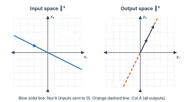
Both sets pass the subspace test, but they live in different places. For an m × n matrix, Nul A sits inside ℝⁿ (inputs have n entries) and Col A sits inside ℝᵐ (outputs have m entries).
Definitions and how to find each space
For an m × n matrix A with columns a₁, …, aₙ:
\operatorname{Nul} A = \{\, x \in \mathbb{R}^n : Ax = \mathbf{0} \,\}\operatorname{Col} A = \operatorname{Span}\{a_1, \dots, a_n\} = \{\, Ax : x \in \mathbb{R}^n \,\}The null space is described implicitly: you get a condition that a vector must pass. The column space is described explicitly: you are handed vectors that build it. So each one has its own easy task and its own harder task.
| Task | Null space | Column space |
|---|---|---|
| Lives in | ℝⁿ (n = number of columns) | ℝᵐ (m = number of rows) |
| Test whether a vector is in it | Compute Au and check for 0 | Row reduce [A | b] and check for consistency |
| Find vectors that span it | Solve Ax = 0 in parametric vector form | Take the pivot columns of the original A |
| It is all of the space when | A = O, the zero matrix | A has a pivot in every row |
| It is just {0} when | A has a pivot in every column | A = O |
To find a spanning set for Nul A:
- Row reduce A to reduced row echelon form. For Ax = 0 the zero column never changes, so you can leave it off.
- Write the equations and solve for the basic variables in terms of the free variables.
- Write the general solution in parametric vector form. The vectors that multiply the free variables span Nul A.
- If there are no free variables, Nul A = {0}.
To describe Col A: the columns of A span it by definition. The pivot columns of the original matrix already span it, because each non-pivot column is a combination of the pivot columns before it. Use the columns of A itself, not the columns of its echelon form.
Null space and column space examples
Example 1: Testing membership
Let A = \begin{bmatrix} 1 & 3 & 5 \\ 2 & 5 & 9 \\ -1 & -1 & -3 \end{bmatrix}. Is u = (4, 2, −2) in Nul A? Is w = (1, 1, 1) in Nul A?
1(4) + 3(2) + 5(-2) = 4 + 6 - 10 = 0
Row 1 of A times u (see matrix equation Ax = b).
2(4) + 5(2) + 9(-2) = 8 + 10 - 18 = 0
Row 2 of A times u.
-1(4) - 1(2) - 3(-2) = -4 - 2 + 6 = 0
Row 3 of A times u.
Au = (0, 0, 0), so u is in Nul A.
1(1) + 3(1) + 5(1) = 9
Row 1 of A times w. The first entry is already not 0.
Answer: u is in Nul A, but w is not, because Aw has first entry 9 ≠ 0. No row reduction is needed to test a vector.
Example 2: A spanning set for the null space
Find vectors that span Nul A for A = \begin{bmatrix} 1 & 2 & -4 & 3 \\ 2 & 5 & -11 & 8 \\ -1 & 1 & -5 & 3 \end{bmatrix}.
\begin{bmatrix} 1 & 2 & -4 & 3 \\ 2 & 5 & -11 & 8 \\ -1 & 1 & -5 & 3 \end{bmatrix}Start with A. The zero column of [A | 0] never changes, so leave it off.
\sim \begin{bmatrix} 1 & 2 & -4 & 3 \\ 0 & 1 & -3 & 2 \\ -1 & 1 & -5 & 3 \end{bmatrix}R₂ − 2R₁ → R₂ (see Gaussian elimination).
\sim \begin{bmatrix} 1 & 2 & -4 & 3 \\ 0 & 1 & -3 & 2 \\ 0 & 3 & -9 & 6 \end{bmatrix}R₃ + R₁ → R₃.
\sim \begin{bmatrix} 1 & 2 & -4 & 3 \\ 0 & 1 & -3 & 2 \\ 0 & 0 & 0 & 0 \end{bmatrix}R₃ − 3R₂ → R₃.
\sim \begin{bmatrix} 1 & 0 & 2 & -1 \\ 0 & 1 & -3 & 2 \\ 0 & 0 & 0 & 0 \end{bmatrix}R₁ − 2R₂ → R₁. This is the reduced row echelon form; x₃ and x₄ are free.
x_1 = -2x_3 + x_4
Row 1 says x₁ + 2x₃ − x₄ = 0. Solve for x₁.
x_2 = 3x_3 - 2x_4
Row 2 says x₂ − 3x₃ + 2x₄ = 0. Solve for x₂.
x = \begin{bmatrix} -2x_3 + x_4 \\ 3x_3 - 2x_4 \\ x_3 \\ x_4 \end{bmatrix}Write the general solution.
= x_3\begin{bmatrix} -2 \\ 3 \\ 1 \\ 0 \end{bmatrix} + x_4\begin{bmatrix} 1 \\ -2 \\ 0 \\ 1 \end{bmatrix}Split by free variable (see parametric vector form).
Answer: Nul A = Span{(−2, 3, 1, 0), (1, −2, 0, 1)}, a plane through the origin in ℝ⁴.
Example 3: The column space as a plane
For the same matrix A, find vectors that span Col A, find an equation for Col A, and decide whether b = (1, 3, 2) and c = (2, 1, 0) are in Col A.
\left[\begin{array}{cccc|c} 1 & 2 & -4 & 3 & b_1 \\ 2 & 5 & -11 & 8 & b_2 \\ -1 & 1 & -5 & 3 & b_3 \end{array}\right]Augment A with a general b = (b₁, b₂, b₃).
\sim \left[\begin{array}{cccc|c} 1 & 2 & -4 & 3 & b_1 \\ 0 & 1 & -3 & 2 & b_2 - 2b_1 \\ -1 & 1 & -5 & 3 & b_3 \end{array}\right]R₂ − 2R₁ → R₂.
\sim \left[\begin{array}{cccc|c} 1 & 2 & -4 & 3 & b_1 \\ 0 & 1 & -3 & 2 & b_2 - 2b_1 \\ 0 & 3 & -9 & 6 & b_3 + b_1 \end{array}\right]R₃ + R₁ → R₃.
\sim \left[\begin{array}{cccc|c} 1 & 2 & -4 & 3 & b_1 \\ 0 & 1 & -3 & 2 & b_2 - 2b_1 \\ 0 & 0 & 0 & 0 & b_3 + b_1 - 3(b_2 - 2b_1) \end{array}\right]R₃ − 3R₂ → R₃.
b_3 + b_1 - 3(b_2 - 2b_1) = b_3 + b_1 - 3b_2 + 6b_1
Distribute the −3 in the last entry (see distributive property).
= 7b_1 - 3b_2 + b_3
Combine like terms.
7b_1 - 3b_2 + b_3 = 0
The system is consistent only when the last row reads 0 = 0.
Pivots are in columns 1 and 2, so the first two columns of A span Col A.
7(1) - 3(3) + 2 = 7 - 9 + 2 = 0
Test b = (1, 3, 2).
7(2) - 3(1) + 0 = 14 - 3 = 11 \ne 0
Test c = (2, 1, 0).
Answer: Col A = Span{(1, 2, −1), (2, 5, 1)}, the plane 7x − 3y + z = 0 in ℝ³. The vector b is in Col A; in fact b = −1(1, 2, −1) + 1(2, 5, 1). The vector c is not in Col A.
Example 4: When Nul A is {0} and Col A is everything
Describe Nul A and Col A for A = \begin{bmatrix} 1 & 2 & 0 \\ 0 & 1 & 3 \\ 2 & 3 & -2 \end{bmatrix}.
\begin{bmatrix} 1 & 2 & 0 \\ 0 & 1 & 3 \\ 2 & 3 & -2 \end{bmatrix}Start with A.
\sim \begin{bmatrix} 1 & 2 & 0 \\ 0 & 1 & 3 \\ 0 & -1 & -2 \end{bmatrix}R₃ − 2R₁ → R₃.
\sim \begin{bmatrix} 1 & 2 & 0 \\ 0 & 1 & 3 \\ 0 & 0 & 1 \end{bmatrix}R₃ + R₂ → R₃. This is an echelon form.
There is a pivot in every column, so Ax = 0 has no free variables and only the trivial solution.
There is a pivot in every row, so Ax = b is consistent for every b in ℝ³.
Answer: Nul A = {0} and Col A = ℝ³. This matches the invertible matrix theorem: A is invertible.
Example 5: Balanced traffic in a one-way network
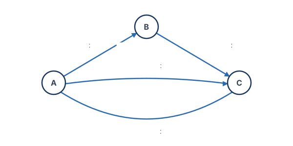
Three intersections A, B and C are joined by four one-way streets: street 1 runs A → B, street 2 runs B → C, street 3 runs C → A, and street 4 runs A → C. Let x₁, …, x₄ be the flows in cars per minute. Traffic is balanced when the flow into each intersection equals the flow out. Find all balanced flows, then find x₁ and x₂ when x₃ = 30 and x₄ = 10.
x_3 - x_1 - x_4 = 0
Intersection A: in (street 3) minus out (streets 1 and 4).
x_1 - x_2 = 0
Intersection B: in (street 1) minus out (street 2).
x_2 + x_4 - x_3 = 0
Intersection C: in (streets 2 and 4) minus out (street 3).
\begin{bmatrix} -1 & 0 & 1 & -1 \\ 1 & -1 & 0 & 0 \\ 0 & 1 & -1 & 1 \end{bmatrix}Balanced flows are the solutions of Mx = 0 for this coefficient matrix M.
\sim \begin{bmatrix} 1 & -1 & 0 & 0 \\ -1 & 0 & 1 & -1 \\ 0 & 1 & -1 & 1 \end{bmatrix}R₁ ↔ R₂.
\sim \begin{bmatrix} 1 & -1 & 0 & 0 \\ 0 & -1 & 1 & -1 \\ 0 & 1 & -1 & 1 \end{bmatrix}R₂ + R₁ → R₂.
\sim \begin{bmatrix} 1 & -1 & 0 & 0 \\ 0 & -1 & 1 & -1 \\ 0 & 0 & 0 & 0 \end{bmatrix}R₃ + R₂ → R₃.
\sim \begin{bmatrix} 1 & -1 & 0 & 0 \\ 0 & 1 & -1 & 1 \\ 0 & 0 & 0 & 0 \end{bmatrix}−1R₂ → R₂.
\sim \begin{bmatrix} 1 & 0 & -1 & 1 \\ 0 & 1 & -1 & 1 \\ 0 & 0 & 0 & 0 \end{bmatrix}R₁ + R₂ → R₁. Now x₃ and x₄ are free.
x_1 = x_3 - x_4,\quad x_2 = x_3 - x_4
Solve rows 1 and 2 for the basic variables.
x = x_3\begin{bmatrix} 1 \\ 1 \\ 1 \\ 0 \end{bmatrix} + x_4\begin{bmatrix} -1 \\ -1 \\ 0 \\ 1 \end{bmatrix}Write the solution in parametric vector form.
x_1 = 30 - 10 = 20,\quad x_2 = 30 - 10 = 20
Substitute x₃ = 30 and x₄ = 10.
Answer: the balanced flows are Nul M = Span{(1, 1, 1, 0), (−1, −1, 0, 1)}. The first vector is one car per minute driving the full loop A → B → C → A; the second moves one car per minute from the route through B onto the shortcut A → C. With x₃ = 30 and x₄ = 10, x₁ = x₂ = 20. Real flows can’t be negative, so the model also needs x₃ ≥ x₄ ≥ 0.
Common mistakes
| Mistake | Example of the error | Fix |
|---|---|---|
| Using the columns of the echelon form for Col A | Saying Col A = Span{(1, 0, 0), (0, 1, 0)} in Example 3 | Row operations change the column space. Use the pivot columns of the original A: (1, 2, −1) and (2, 5, 1). |
| Putting the null space in the wrong space | Saying Nul A is in ℝ³ for a 3 × 4 matrix | Nul A holds inputs, so it lives in ℝⁿ, where n is the number of columns: here ℝ⁴. |
| Dropping the free-variable entries | Writing (−2, 3) instead of (−2, 3, 1, 0) | Every null space vector has one entry per column, free variables included. |
| Saying the null space is empty | “Ax = 0 has only the trivial solution, so Nul A has nothing in it” | Nul A always contains 0. In that case Nul A = {0}. |
| Row reducing to test one vector | Row reducing A to check whether u is in Nul A | Just compute Au. Row reduction is needed for Col A membership, not Nul A membership. |
Related ideas
Kernel and range. For a linear transformation T(x) = Ax, the kernel of T is Nul A and the range of T is Col A. So T is one-to-one exactly when Nul A = {0}, and T is onto exactly when Col A = ℝᵐ (see one-to-one and onto transformations).
Linear independence. Nul A = {0} means the only weights that make x₁a₁ + ⋯ + xₙaₙ = 0 are all zero, so the columns of A are linearly independent. A nonzero vector in Nul A lists the weights of a dependence among the columns: in Example 1, u = (4, 2, −2) says 4a₁ + 2a₂ − 2a₃ = 0.
Solving Ax = b. Ax = b has a solution exactly when b is in Col A. When it does, every solution is one particular solution plus a vector from Nul A, so the null space measures how much freedom the solutions have. The next lesson, Basis and Dimension, shows that the spanning sets found here are as small as possible.
Practice problems
- Let A = \begin{bmatrix} 2 & 6 \\ 1 & 3 \end{bmatrix}. Is (3, −1) in Nul A?
- For the same A, is (5, 10) in Col A?
- Find vectors that span Nul A for A = \begin{bmatrix} 1 & -2 & 4 \end{bmatrix}.
- Find vectors that span Nul A for A = \begin{bmatrix} 1 & 2 & -1 \\ 3 & 7 & 2 \end{bmatrix}.
- For the matrix in Problem 4, describe Col A.
- Find vectors that span Nul A for the matrix A in Example 1.
- For the matrix A in Example 1, is b = (1, 1, 1) in Col A? If so, write b as a combination of the columns.
- A is a 5 × 7 matrix. Nul A is a subspace of which ℝᵏ? Col A is a subspace of which ℝᵏ?
- Find a matrix A whose null space is the plane x − 2y + 5z = 0 in ℝ³, and a matrix B whose column space is Span{(1, 0, 2), (0, 1, −1)}.
- Find the kernel and range of the linear transformation T(x₁, x₂, x₃) = (x₁ − x₃, x₂ + 2x₃).
Show answers
1.
2(3) + 6(-1) = 6 - 6 = 0
Row 1 of A times (3, −1).
1(3) + 3(-1) = 3 - 3 = 0
Row 2 of A times (3, −1).
Answer: yes. A(3, −1) = (0, 0), so (3, −1) is in Nul A.
2.
\begin{bmatrix} 6 \\ 3 \end{bmatrix} = 3\begin{bmatrix} 2 \\ 1 \end{bmatrix}The second column is 3 times the first, so Col A = Span{(2, 1)}.
c\begin{bmatrix} 2 \\ 1 \end{bmatrix} = \begin{bmatrix} 5 \\ 10 \end{bmatrix}Look for a scalar c.
2c = 5 \Rightarrow c = \tfrac{5}{2}First entries: divide by 2.
c = 10
Second entries.
\tfrac{5}{2} \ne 10The two values of c disagree.
Answer: no. (5, 10) is not a multiple of (2, 1), so it is not in Col A.
3.
x_1 - 2x_2 + 4x_3 = 0
The single equation; x₂ and x₃ are free.
x_1 = 2x_2 - 4x_3
Solve for x₁.
x = x_2\begin{bmatrix} 2 \\ 1 \\ 0 \end{bmatrix} + x_3\begin{bmatrix} -4 \\ 0 \\ 1 \end{bmatrix}Parametric vector form.
Answer: Nul A = Span{(2, 1, 0), (−4, 0, 1)}, a plane in ℝ³.
4.
\begin{bmatrix} 1 & 2 & -1 \\ 3 & 7 & 2 \end{bmatrix} \sim \begin{bmatrix} 1 & 2 & -1 \\ 0 & 1 & 5 \end{bmatrix}R₂ − 3R₁ → R₂.
\sim \begin{bmatrix} 1 & 0 & -11 \\ 0 & 1 & 5 \end{bmatrix}R₁ − 2R₂ → R₁. x₃ is free.
x_1 = 11x_3,\quad x_2 = -5x_3
Solve rows 1 and 2.
x = x_3\begin{bmatrix} 11 \\ -5 \\ 1 \end{bmatrix}Parametric vector form.
Answer: Nul A = Span{(11, −5, 1)}, a line in ℝ³.
5.
\begin{bmatrix} 1 & 2 & -1 \\ 0 & 1 & 5 \end{bmatrix}The echelon form from Problem 4 has a pivot in both rows.
Answer: Ax = b is consistent for every b in ℝ², so Col A = ℝ². The pivot columns (1, 3) and (2, 7) already span it.
6.
\sim \begin{bmatrix} 1 & 3 & 5 \\ 0 & -1 & -1 \\ -1 & -1 & -3 \end{bmatrix}R₂ − 2R₁ → R₂.
\sim \begin{bmatrix} 1 & 3 & 5 \\ 0 & -1 & -1 \\ 0 & 2 & 2 \end{bmatrix}R₃ + R₁ → R₃.
\sim \begin{bmatrix} 1 & 3 & 5 \\ 0 & -1 & -1 \\ 0 & 0 & 0 \end{bmatrix}R₃ + 2R₂ → R₃.
\sim \begin{bmatrix} 1 & 3 & 5 \\ 0 & 1 & 1 \\ 0 & 0 & 0 \end{bmatrix}−1R₂ → R₂.
\sim \begin{bmatrix} 1 & 0 & 2 \\ 0 & 1 & 1 \\ 0 & 0 & 0 \end{bmatrix}R₁ − 3R₂ → R₁. x₃ is free.
x_1 = -2x_3,\quad x_2 = -x_3
Solve rows 1 and 2.
x = x_3\begin{bmatrix} -2 \\ -1 \\ 1 \end{bmatrix}Parametric vector form.
Answer: Nul A = Span{(−2, −1, 1)}, a line in ℝ³. The vector u = (4, 2, −2) from Example 1 is −2 times this vector.
7.
c_1\begin{bmatrix} 1 \\ 2 \\ -1 \end{bmatrix} + c_2\begin{bmatrix} 3 \\ 5 \\ -1 \end{bmatrix} = \begin{bmatrix} 1 \\ 1 \\ 1 \end{bmatrix}Problem 6 shows pivots in columns 1 and 2, so use those columns.
\left[\begin{array}{cc|c} 1 & 3 & 1 \\ 2 & 5 & 1 \\ -1 & -1 & 1 \end{array}\right] \sim \left[\begin{array}{cc|c} 1 & 3 & 1 \\ 0 & -1 & -1 \\ -1 & -1 & 1 \end{array}\right]R₂ − 2R₁ → R₂.
\sim \left[\begin{array}{cc|c} 1 & 3 & 1 \\ 0 & -1 & -1 \\ 0 & 2 & 2 \end{array}\right]R₃ + R₁ → R₃.
\sim \left[\begin{array}{cc|c} 1 & 3 & 1 \\ 0 & -1 & -1 \\ 0 & 0 & 0 \end{array}\right]R₃ + 2R₂ → R₃. The system is consistent.
c_2 = 1
Row 2: −c₂ = −1.
c_1 = 1 - 3(1) = -2
Row 1: c₁ = 1 − 3c₂.
-2\begin{bmatrix} 1 \\ 2 \\ -1 \end{bmatrix} + 1\begin{bmatrix} 3 \\ 5 \\ -1 \end{bmatrix} = \begin{bmatrix} -2 + 3 \\ -4 + 5 \\ 2 - 1 \end{bmatrix} = \begin{bmatrix} 1 \\ 1 \\ 1 \end{bmatrix}Check.
Answer: yes. b = −2a₁ + a₂ (+ 0a₃).
8.
Nul A holds the inputs, which have 7 entries. Col A holds the outputs, which have 5 entries.
Answer: Nul A is a subspace of ℝ⁷ and Col A is a subspace of ℝ⁵.
9.
A = \begin{bmatrix} 1 & -2 & 5 \end{bmatrix}Ax = 0 is exactly the equation x − 2y + 5z = 0.
B = \begin{bmatrix} 1 & 0 \\ 0 & 1 \\ 2 & -1 \end{bmatrix}Use the two given vectors as the columns.
Answer: A = [1 −2 5] works, and B with columns (1, 0, 2) and (0, 1, −1) works. Other answers are possible.
10.
\begin{bmatrix} 1 & 0 & -1 \\ 0 & 1 & 2 \end{bmatrix}The standard matrix of T. It is already in reduced row echelon form, and x₃ is free.
x_1 = x_3,\quad x_2 = -2x_3
Solve rows 1 and 2 of Ax = 0.
x = x_3\begin{bmatrix} 1 \\ -2 \\ 1 \end{bmatrix}Parametric vector form.
Answer: the kernel of T is Span{(1, −2, 1)}, a line in ℝ³. There is a pivot in both rows, so the range of T is all of ℝ².
Null space and column space FAQ
What is the difference between the null space and the column space?
The null space is the set of inputs x with Ax = 0, and it lives in ℝⁿ. The column space is the set of all outputs Ax, which is the span of the columns, and it lives in ℝᵐ.
Is the null space the same as the kernel?
Yes, for a matrix. The kernel of the transformation T(x) = Ax is exactly Nul A, and the range of T is Col A. “Kernel” is also used for linear transformations between other vector spaces.
How do you find the null space of a matrix?
Row reduce A to reduced row echelon form, solve Ax = 0 for the basic variables, and write the solution in parametric vector form. The vectors that multiply the free variables span the null space.
Can the null space be just the zero vector?
Yes. Nul A = {0} exactly when A has a pivot in every column, which means the columns of A are linearly independent.
Summary
- Nul A is the set of solutions of Ax = 0; it is a subspace of ℝⁿ.
- Col A is the span of the columns of A, the set of all outputs Ax; it is a subspace of ℝᵐ.
- To test a vector for Nul A, compute Au. To test b for Col A, check whether Ax = b is consistent.
- The vectors in the parametric vector form of the solution of Ax = 0 span Nul A. The pivot columns of the original A span Col A.
- Nul A = {0} when there is a pivot in every column; Col A = ℝᵐ when there is a pivot in every row.
Previous lesson: Subspaces
Next lesson: Basis and Dimension
Back to the Linear Algebra Index