
Linear Approximation
Linear approximation estimates a function’s value with its tangent line. Near a point x = a where you know f(a) and f′(a), use the linearization L(x) = f(a) + f'(a)(x - a). For x close to a, f(x) \approx L(x). For example, starting from the exact value \sqrt{25} = 5, it gives the estimate \sqrt{26} \approx 5.1.
Before this lesson: Equation of a Tangent Line, Power Rule and Chain Rule
The idea: zoom in on a curve
If you zoom in far enough on a smooth curve, it looks almost straight. The straight line it looks like is the tangent line. So near the point of tangency, the tangent line’s height is a good stand-in for the function’s height.
That is useful when f(x) is hard to compute but f(a) is easy. To estimate \sqrt{26}, start at a = 25, where \sqrt{25} = 5 is exact, and follow the tangent line a little way.
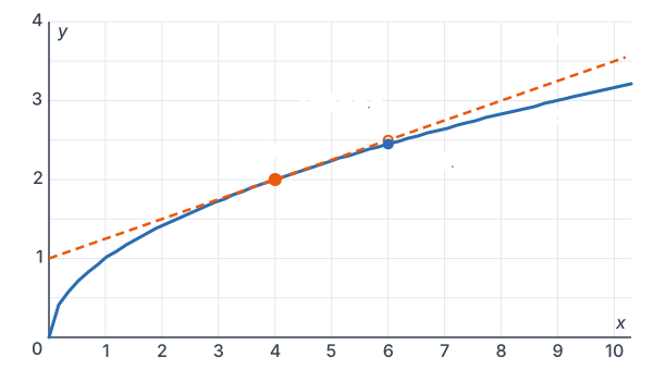
The linearization formula
L(x) = f(a) + f'(a)(x - a), \qquad f(x) \approx L(x) \text{ for } x \text{ near } aL(x) is the tangent line at x = a written in point-slope form. The term f′(a)(x − a) is the rise along the tangent line from a to x.
- Pick a value a close to x where f(a) is easy to find exactly.
- Find f(a) and f′(a).
- Write L(x) = f(a) + f′(a)(x − a).
- Substitute the x you want to estimate.
Over or under? If the graph is concave down near a (it bends like a cap, f'' \lt 0), the tangent line lies above the curve, so L(x) is an overestimate. If it is concave up (a cup, f'' \gt 0), L(x) is an underestimate.
Linear approximation examples
Example 1: Estimate a square root
Use a linear approximation to estimate \sqrt{26}.
f(x) = \sqrt{x}, \; a = 25Choose a = 25, the nearest perfect square.
f(25) = 5
Find f(a).
f'(x) = \frac{1}{2\sqrt{x}} \Rightarrow f'(25) = \frac{1}{10}Differentiate x^(1/2) and evaluate at 25.
L(x) = 5 + \frac{1}{10}(x - 25)Write the linearization.
L(26) = 5 + \frac{1}{10}(1) = 5.1Substitute x = 26.
Answer: \sqrt{26} \approx 5.1. The true value is about 5.0990, so the estimate is off by only 0.001. It is a little high because \sqrt{x} is concave down.
Example 2: The small-angle approximation
Find the linearization of f(x) = \sin x at a = 0, and use it to estimate sin(0.1).
f(0) = \sin 0 = 0
Find f(a).
f'(x) = \cos x \Rightarrow f'(0) = 1
Differentiate and evaluate at 0.
L(x) = 0 + 1(x - 0) = x
Write the linearization.
\sin(0.1) \approx L(0.1) = 0.1
Substitute x = 0.1 (radians).
Answer: \sin x \approx x near 0, so \sin(0.1) \approx 0.1. The true value is 0.09983. Physics uses this approximation for small swings of a pendulum.
Example 3: A power near 1
Estimate (1.02)^5.
f(x) = x^5, \; a = 1
1.02 is close to 1, and 1⁵ = 1.
f(1) = 1, \; f'(x) = 5x^4 \Rightarrow f'(1) = 5
Find f(a) and f′(a).
L(x) = 1 + 5(x - 1)
Write the linearization.
L(1.02) = 1 + 5(0.02) = 1.1
Substitute x = 1.02.
Answer: (1.02)^5 \approx 1.1. The true value is 1.10408. This is why 2% growth for 5 years is roughly 10% in total.
Example 4: A cube root
Estimate \sqrt[3]{8.3}.
f(x) = x^{1/3}, \; a = 88 is a perfect cube near 8.3.
f(8) = 2
Find f(a).
f'(x) = \frac{1}{3}x^{-2/3}Power rule.
f'(8) = \frac{1}{3} \cdot \frac{1}{4} = \frac{1}{12}8^{-2/3} = \frac{1}{(\sqrt[3]{8})^2} = \frac{1}{4}.
L(8.3) = 2 + \frac{1}{12}(0.3) = 2 + 0.025 = 2.025Substitute x = 8.3.
Answer: \sqrt[3]{8.3} \approx 2.025. The true value is about 2.02469.
Example 5: Word problem with temperature
At 10 minutes after an oven is turned on, a sensor reads 350°F, and the temperature is rising 12°F per minute. Estimate the temperature at 10.5 minutes.
T(10) = 350, \; T'(10) = 12
The value and the rate at a = 10.
L(t) = 350 + 12(t - 10)
Write the linearization.
L(10.5) = 350 + 12(0.5) = 356
Substitute t = 10.5.
Answer: about 356°F. You don’t need a formula for T(t) at all, only its value and rate at one moment. The estimate gets worse further from t = 10, because the rate itself changes as the oven nears its set temperature.
Common mistakes
| Mistake | Example of the error | Fix |
|---|---|---|
| Evaluating f′ at x instead of a | For √26, using f′(26) | Use f′(a) = f′(25) = 1/10. You don’t know f at 26; that’s the point. |
| Choosing a far from x | Estimating √26 from a = 16 | Choose the nearest easy value, here a = 25. |
| Forgetting the (x − a) | L(x) = f(a) + f'(a)x | The slope multiplies the distance from a: f′(a)(x − a). |
| Using degrees in trig approximations | \sin(6^\circ) \approx 6 | Convert to radians: 6° ≈ 0.1047, so sin 6° ≈ 0.1047. |
| Calling every estimate an overestimate | Saying (1.02)⁵ ≈ 1.1 is too high | x⁵ is concave up near 1, so the tangent line is below the curve: 1.1 is an underestimate. |
Related methods
Differentials
The change along the tangent line, f′(a)Δx, is called a differential. Differentials estimate how much a quantity changes, such as the error in a volume caused by a small error in a measurement. That is the next lesson, Differentials.
Newton’s method
Following a tangent line down to where it crosses the x-axis gives an estimate of a zero of f. Repeating this is Newton’s method, which comes later in Calculus 1.
Practice problems
- Find the linearization of f(x) = x^3 at a = 2.
- Estimate \sqrt{99}.
- Estimate (2.01)^4.
- Estimate \frac{1}{1.05}.
- Estimate ln(1.04).
- Estimate e^{-0.03}.
- Estimate \sqrt[3]{27.5}.
- Find the linearization of tan x at a = \frac{\pi}{4} and use it to estimate tan(0.8).
- Is your estimate of \sqrt{99} in Problem 2 an overestimate or an underestimate? Explain.
- A car passes a marker 120 m down the road at t = 4 s, moving at 25 m/s. Estimate its position at t = 4.2 s.
Show answers
1.
f(2) = 8
Find f(a).
f'(x) = 3x^2 \Rightarrow f'(2) = 12
Differentiate and evaluate at 2.
L(x) = 8 + 12(x - 2)
Write the linearization.
L(x) = 12x - 16
Distribute and combine like terms.
Answer: L(x) = 12x - 16
2.
f(100) = 10, \; f'(100) = \frac{1}{2\sqrt{100}} = \frac{1}{20}Use f(x) = √x and a = 100.
L(99) = 10 + \frac{1}{20}(-1) = 9.95Substitute x = 99.
Answer: √99 ≈ 9.95
3.
f(2) = 16, \; f'(2) = 4(2)^3 = 32
Use f(x) = x⁴ and a = 2.
L(2.01) = 16 + 32(0.01) = 16.32
Substitute x = 2.01.
Answer: about 16.32
4.
f(1) = 1, \; f'(x) = -x^{-2} \Rightarrow f'(1) = -1Use f(x) = 1/x and a = 1.
L(1.05) = 1 - 1(0.05) = 0.95
Substitute x = 1.05.
Answer: about 0.95
5.
f(1) = \ln 1 = 0, \; f'(1) = \frac{1}{1} = 1Use f(x) = ln x and a = 1.
L(1.04) = 0 + 1(0.04) = 0.04
Substitute x = 1.04.
Answer: ln(1.04) ≈ 0.04
6.
f(0) = e^0 = 1, \; f'(0) = e^0 = 1
Use f(x) = eˣ and a = 0.
L(-0.03) = 1 + 1(-0.03) = 0.97
Substitute x = −0.03.
Answer: about 0.97
7.
f(27) = 3, \; f'(27) = \frac{1}{3}(27)^{-2/3} = \frac{1}{27}Use f(x) = x^(1/3) and a = 27; 27^(2/3) = 9.
L(27.5) = 3 + \frac{1}{27}(0.5) = 3 + \frac{1}{54} \approx 3.0185Substitute x = 27.5.
Answer: about 3.0185
8.
f\left(\frac{\pi}{4}\right) = 1, \; f'\left(\frac{\pi}{4}\right) = \sec^2\frac{\pi}{4} = 2tan(π/4) = 1 and sec(π/4) = √2.
L(x) = 1 + 2\left(x - \frac{\pi}{4}\right)Write the linearization.
L(0.8) = 1 + 2(0.8 - 0.7854) \approx 1.0292
Substitute x = 0.8, with π/4 ≈ 0.7854.
Answer: tan(0.8) ≈ 1.0292
9.
f''(x) = -\frac{1}{4}x^{-3/2}Differentiate f′(x) = ½ x^(−1/2) again.
f''(100) = -\frac{1}{4000}Evaluate at a = 100: 100^(3/2) = 1000. It is negative.
Answer: an overestimate. √x is concave down, so its tangent line lies above the curve. (The true value is 9.94987.)
10.
s(4) = 120, \; s'(4) = 25
Position and velocity at a = 4.
L(4.2) = 120 + 25(0.2) = 125
Substitute t = 4.2.
Answer: about 125 m
Linear approximation FAQ
What is the linear approximation formula?
L(x) = f(a) + f'(a)(x - a). It is the tangent line at x = a, used to estimate f(x) for x near a.
Is linear approximation the same as linearization?
Yes. The linearization is the function L(x), and linear approximation means using L(x) in place of f(x).
How do you know if a linear approximation is an over- or underestimate?
Check concavity at a. If f″(a) is negative, the estimate is too high. If f″(a) is positive, it is too low.
How accurate is a linear approximation?
It is very accurate close to a and gets worse farther away. How fast it gets worse depends on how much the graph bends there.
Summary
- L(x) = f(a) + f'(a)(x - a) is the tangent line at a.
- Use f(x) \approx L(x) for x near a, where f(a) is easy to find.
- Concave down: overestimate. Concave up: underestimate.
- Familiar results: \sin x \approx x, e^x \approx 1 + x and \ln(1 + x) \approx x near 0.
- The estimate is only good near a.
Previous lesson: Related Rates
Next lesson: Differentials
Back to the Calculus 1 Index