Least-Squares Solutions: Normal Equations

A least-squares solution of Ax = b is a vector x̂ that makes Ax̂ as close to b as possible, even when Ax = b has no exact solution. You find it by solving the normal equations AᵀAx̂ = Aᵀb. Then Ax̂ is the projection of b onto the column space of A.

Before this lesson: Orthogonal Projections, Transpose of a Matrix and Inverse Matrices

What a least-squares solution means

Data rarely fit a model exactly, so a system like Ax = b often has no solution. Every vector Ax lies in the column space of A, and b sits outside it. The best you can do is pick the x that brings Ax closest to b.

“Closest” means the length ‖b − Ax‖ is as small as possible. That length is the square root of a sum of squares, which is where the name “least squares” comes from. The closest point in the column space is the orthogonal projection of b, so Ax̂ = proj b.

Scatter plot of test score against hours studied for four students: (1, 60), (2, 70), (4, 75) and (5, 85). The least-squares line y-hat = 56 + 5.5x passes between the points. Dashed vertical segments show the residuals −1.5, 3, −3 and 1.5, the vertical gaps between each point and the line. — The least-squares solution (56, 5.5) gives the line whose squared residuals add up to 22.5, the smallest total possible.

The normal equations

The leftover part b − Ax̂ must be orthogonal to every column of A. In matrix form that says Aᵀ(b − Ax̂) = 0, which rearranges to

A^T A\,\hat{x} = A^T b

These are the normal equations. Their solutions are exactly the least-squares solutions of Ax = b.
If the columns of A are linearly independent, then AᵀA is invertible and there is exactly one least-squares solution, x̂ = (AᵀA)⁻¹Aᵀb.
If the columns are dependent, there are infinitely many least-squares solutions, but Ax̂ is the same for all of them.
The least-squares error is ‖b − Ax̂‖. The vector r = b − Ax̂ is called the residual.
If Ax = b has an exact solution, the least-squares solution is that solution and the error is 0.

How to find a least-squares solution

Compute AᵀA and Aᵀb.
Solve AᵀAx̂ = Aᵀb by row reduction or, for a 2 × 2 system, with the inverse.
Find Ax̂ and the residual r = b − Ax̂.
Check that Aᵀr = 0. Find ‖r‖ if you need the least-squares error.

Least-squares solution examples

Example 1: An inconsistent system

Find the least-squares solution of Ax = b, where $A = \begin{bmatrix} 1 & 0 \\ 0 & 1 \\ 1 & 1 \end{bmatrix}$ and $b = \begin{bmatrix} 1 \\ 2 \\ 6 \end{bmatrix}$ . Then find the least-squares error.

x_1 = 1,\ x_2 = 2,\ x_1 + x_2 = 6

The system has no solution, because 1 + 2 is not 6.

A^T A = \begin{bmatrix} 1 & 0 & 1 \\ 0 & 1 & 1 \end{bmatrix}\begin{bmatrix} 1 & 0 \\ 0 & 1 \\ 1 & 1 \end{bmatrix} = \begin{bmatrix} 1 + 0 + 1 & 0 + 0 + 1 \\ 0 + 0 + 1 & 0 + 1 + 1 \end{bmatrix} = \begin{bmatrix} 2 & 1 \\ 1 & 2 \end{bmatrix}

Multiply Aᵀ by A (see matrix multiplication).

A^T b = \begin{bmatrix} 1 + 0 + 6 \\ 0 + 2 + 6 \end{bmatrix} = \begin{bmatrix} 7 \\ 8 \end{bmatrix}

Multiply Aᵀ by b.

(A^T A)^{-1} = \frac{1}{4 - 1}\begin{bmatrix} 2 & -1 \\ -1 & 2 \end{bmatrix} = \frac{1}{3}\begin{bmatrix} 2 & -1 \\ -1 & 2 \end{bmatrix}

Invert the 2 × 2 matrix (see inverse matrices).

\hat{x} = \frac{1}{3}\begin{bmatrix} 14 - 8 \\ -7 + 16 \end{bmatrix} = \frac{1}{3}\begin{bmatrix} 6 \\ 9 \end{bmatrix} = \begin{bmatrix} 2 \\ 3 \end{bmatrix}

Multiply the inverse by Aᵀb.

A\hat{x} = (2, 3, 5),\quad r = b - A\hat{x} = (1 - 2,\ 2 - 3,\ 6 - 5) = (-1, -1, 1)

Closest point and residual.

A^T r = (-1 + 0 + 1,\ 0 - 1 + 1) = (0, 0)

Check: r is orthogonal to both columns.

\|r\| = \sqrt{1 + 1 + 1} = \sqrt{3}

Least-squares error.

Answer: x̂ = (2, 3), and the least-squares error is √3 ≈ 1.73.

Example 2: Orthogonal columns

Find the least-squares solution of Ax = b for $A = \begin{bmatrix} 1 & -1 \\ 1 & 0 \\ 1 & 1 \end{bmatrix}$ and $b = \begin{bmatrix} 2 \\ 3 \\ 7 \end{bmatrix}$ .

A^T A = \begin{bmatrix} 1 + 1 + 1 & -1 + 0 + 1 \\ -1 + 0 + 1 & 1 + 0 + 1 \end{bmatrix} = \begin{bmatrix} 3 & 0 \\ 0 & 2 \end{bmatrix}

The columns are orthogonal, so AᵀA is diagonal.

A^T b = \begin{bmatrix} 2 + 3 + 7 \\ -2 + 0 + 7 \end{bmatrix} = \begin{bmatrix} 12 \\ 5 \end{bmatrix}

Multiply Aᵀ by b.

3\hat{x}_1 = 12 \;\Rightarrow\; \hat{x}_1 = 4,\qquad 2\hat{x}_2 = 5 \;\Rightarrow\; \hat{x}_2 = 2.5

Each equation has one unknown.

A\hat{x} = (4 - 2.5,\ 4,\ 4 + 2.5) = (1.5, 4, 6.5)

Closest point.

r = (2 - 1.5,\ 3 - 4,\ 7 - 6.5) = (0.5, -1, 0.5)

Residual.

A^T r = (0.5 - 1 + 0.5,\ -0.5 + 0 + 0.5) = (0, 0)

Check.

Answer: x̂ = (4, 2.5). With orthogonal columns, each weight is just (b · aᵢ)/(aᵢ · aᵢ), as in Orthogonal Projections.

Example 3: Best-fit line for study hours and scores

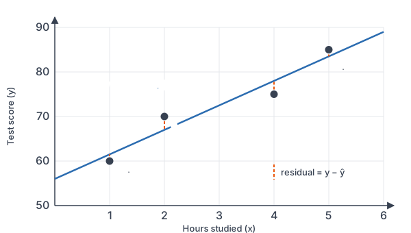
A tutor records hours studied x and test scores y for four students: (1, 60), (2, 70), (4, 75) and (5, 85). Find the least-squares line y = c + mx, and predict the score for 3 hours of study.

A = \begin{bmatrix} 1 & 1 \\ 1 & 2 \\ 1 & 4 \\ 1 & 5 \end{bmatrix},\quad b = \begin{bmatrix} 60 \\ 70 \\ 75 \\ 85 \end{bmatrix},\quad \hat{x} = \begin{bmatrix} c \\ m \end{bmatrix}

Each point gives one equation c + mx = y.

A^T A = \begin{bmatrix} 4 & 1 + 2 + 4 + 5 \\ 12 & 1 + 4 + 16 + 25 \end{bmatrix} = \begin{bmatrix} 4 & 12 \\ 12 & 46 \end{bmatrix}

Count, sum of x and sum of x².

A^T b = \begin{bmatrix} 60 + 70 + 75 + 85 \\ 60 + 140 + 300 + 425 \end{bmatrix} = \begin{bmatrix} 290 \\ 925 \end{bmatrix}

Sum of y and sum of xy.

(A^T A)^{-1} = \frac{1}{184 - 144}\begin{bmatrix} 46 & -12 \\ -12 & 4 \end{bmatrix} = \frac{1}{40}\begin{bmatrix} 46 & -12 \\ -12 & 4 \end{bmatrix}

Invert. The determinant is 4(46) − 12(12) = 40.

\hat{x} = \frac{1}{40}\begin{bmatrix} 13340 - 11100 \\ -3480 + 3700 \end{bmatrix} = \frac{1}{40}\begin{bmatrix} 2240 \\ 220 \end{bmatrix} = \begin{bmatrix} 56 \\ 5.5 \end{bmatrix}

Multiply by Aᵀb.

r = (60 - 61.5,\ 70 - 67,\ 75 - 78,\ 85 - 83.5) = (-1.5, 3, -3, 1.5)

Residuals: data minus the line’s values.

56 + 5.5(3) = 56 + 16.5 = 72.5

Predict for x = 3.

Answer: the least-squares line is y = 56 + 5.5x, and it predicts a score of 72.5 for 3 hours. This is the same line as the least-squares regression line from statistics.

Example 4: Fitting a parabola

A farmer tests four fertilizer levels, coded t = −2, −1, 1, 2 so that 0 is the standard amount. The yields are 7, 13, 23 and 17 kg per row. Find the least-squares parabola y = a + bt + ct².

A = \begin{bmatrix} 1 & -2 & 4 \\ 1 & -1 & 1 \\ 1 & 1 & 1 \\ 1 & 2 & 4 \end{bmatrix},\quad b = \begin{bmatrix} 7 \\ 13 \\ 23 \\ 17 \end{bmatrix}

Columns 1, t and t².

A^T A = \begin{bmatrix} 4 & 0 & 10 \\ 0 & 10 & 0 \\ 10 & 0 & 34 \end{bmatrix}

The sums of t and t³ are 0 because the t values are symmetric.

A^T b = \begin{bmatrix} 7 + 13 + 23 + 17 \\ -14 - 13 + 23 + 34 \\ 28 + 13 + 23 + 68 \end{bmatrix} = \begin{bmatrix} 60 \\ 30 \\ 132 \end{bmatrix}

Multiply Aᵀ by b.

10b = 30 \;\Rightarrow\; b = 3

The middle equation has only b.

4a + 10c = 60 \;\Rightarrow\; 2a + 5c = 30

First equation, divided by 2.

10a + 34c = 132

Third equation.

10a + 25c = 150

Multiply 2a + 5c = 30 by 5.

9c = -18 \;\Rightarrow\; c = -2

Subtract the two equations (as in the elimination method), then divide by 9.

2a + 5(-2) = 30 \;\Rightarrow\; 2a = 40 \;\Rightarrow\; a = 20

Substitute c = −2 and solve.

r = (7 - 6,\ 13 - 15,\ 23 - 21,\ 17 - 18) = (1, -2, 2, -1)

Residuals, using the model values 6, 15, 21 and 18.

Answer: y = 20 + 3t − 2t². The residuals are small, and Aᵀr = 0 checks: 1 − 2 + 2 − 1 = 0, −2 + 2 + 2 − 2 = 0 and 4 − 2 + 2 − 4 = 0.

Example 5: Dependent columns

Find all least-squares solutions of Ax = b for $A = \begin{bmatrix} 1 & 2 \\ 1 & 2 \\ 1 & 2 \end{bmatrix}$ and $b = \begin{bmatrix} 1 \\ 4 \\ 7 \end{bmatrix}$ .

A^T A = \begin{bmatrix} 3 & 6 \\ 6 & 12 \end{bmatrix},\quad A^T b = \begin{bmatrix} 12 \\ 24 \end{bmatrix}

Column 2 is twice column 1, so AᵀA is not invertible.

\left[\begin{array}{cc|c} 3 & 6 & 12 \\ 6 & 12 & 24 \end{array}\right] \sim \left[\begin{array}{cc|c} 1 & 2 & 4 \\ 0 & 0 & 0 \end{array}\right]

R₂ − 2R₁, then (1/3)R₁ (see Gaussian elimination).

\hat{x}_1 = 4 - 2\hat{x}_2

x̂₂ is free.

\hat{x} = \begin{bmatrix} 4 \\ 0 \end{bmatrix} + t\begin{bmatrix} -2 \\ 1 \end{bmatrix}

Write the solutions in parametric vector form.

A\hat{x} = (4 - 2t + 2t)(1, 1, 1) = (4, 4, 4)

Every solution gives the same closest point.

Answer: x̂ = (4, 0) + t(−2, 1) for any t, and Ax̂ = (4, 4, 4) every time. The closest point puts the average of 1, 4 and 7 in each entry.

Common mistakes

Mistake	Example of the error	Fix
Stopping when Ax = b has no solution	Row reducing Example 1 and answering “no solution”	When the question asks for a least-squares solution, solve AᵀAx̂ = Aᵀb instead.
Leaving Aᵀ off the right side	Writing AᵀAx̂ = b in Example 1, a 2 × 2 matrix times x̂ equal to a vector in ℝ³	Multiply both sides by Aᵀ: the right side is Aᵀb = (7, 8).
Inverting AᵀA when the columns are dependent	Using (AᵀA)⁻¹ in Example 5, where det AᵀA = 36 − 36 = 0	Row reduce the normal equations and write every solution with a free variable.
Giving Ax̂ as the answer	Answering (2, 3, 5) in Example 1	x̂ = (2, 3) is the solution. Ax̂ = (2, 3, 5) is the closest point to b.
Reporting ‖r‖² as the error	Saying the error in Example 1 is 3	The least-squares error is ‖r‖ = √3. The sum of squares is 3.

Related methods

With QR. If A = QR, the normal equations become Rx̂ = Qᵀb, a triangular system. This avoids forming AᵀA and is more accurate on a computer. See QR factorization.

With orthogonal columns. As in Example 2, AᵀA is diagonal, so each entry of x̂ comes from one dot product.

With statistics formulas. For a straight line, the normal equations give the slope and intercept formulas of the least-squares regression line. The matrix method also handles parabolas and models with several inputs.

Practice problems

Find the least-squares solution of Ax = b for A = [1 0; 0 1; 1 1] and b = (3, 1, 2).
Find the least-squares error for Problem 1.
Find the least-squares solution for A = [1 −1; 1 0; 1 1] and b = (1, 1, 4).
Find the least-squares line y = c + mx for the points (0, 1), (1, 1), (2, 3) and (3, 4).
Find the least-squares solution for A = [1 0; 0 1; 1 1] and b = (1, 2, 3). What is the error, and why?
Check that the residual r = (−1.5, 3, −3, 1.5) from Example 3 satisfies Aᵀr = 0.
Find all least-squares solutions for A = [1 1; 2 2] and b = (1, 1).
Find the least-squares parabola y = a + bt + ct² for t = −2, −1, 1, 2 and y = 8, 3, 9, 10.
Find the least-squares solution of the three equations x = 3, x = 5 and x = 10.
A lemonade stand charged $1, $2, $3 and $4 and sold 9, 8, 4 and 3 dozen cups. Find the least-squares line for dozens sold y against price x.

Show answers

A^T A = \begin{bmatrix} 2 & 1 \\ 1 & 2 \end{bmatrix},\quad A^T b = \begin{bmatrix} 3 + 2 \\ 1 + 2 \end{bmatrix} = \begin{bmatrix} 5 \\ 3 \end{bmatrix}

Normal equations.

\hat{x} = \frac{1}{3}\begin{bmatrix} 10 - 3 \\ -5 + 6 \end{bmatrix} = \begin{bmatrix} 7/3 \\ 1/3 \end{bmatrix}

Multiply by (AᵀA)⁻¹ from Example 1.

Answer: x̂ = (7/3, 1/3).

A\hat{x} = \left(\tfrac{7}{3}, \tfrac{1}{3}, \tfrac{8}{3}\right),\quad r = \left(\tfrac{2}{3}, \tfrac{2}{3}, -\tfrac{2}{3}\right)

Closest point and residual.

\|r\| = \sqrt{\tfrac{4}{9} + \tfrac{4}{9} + \tfrac{4}{9}} = \sqrt{\tfrac{12}{9}} = \tfrac{2\sqrt{3}}{3}

Length (see simplifying square roots).

Answer: the error is 2√3/3 ≈ 1.15.

A^T A = \begin{bmatrix} 3 & 0 \\ 0 & 2 \end{bmatrix},\quad A^T b = \begin{bmatrix} 1 + 1 + 4 \\ -1 + 0 + 4 \end{bmatrix} = \begin{bmatrix} 6 \\ 3 \end{bmatrix}

Normal equations.

3\hat{x}_1 = 6,\quad 2\hat{x}_2 = 3

Diagonal system.

Answer: x̂ = (2, 1.5).

A^T A = \begin{bmatrix} 4 & 6 \\ 6 & 14 \end{bmatrix},\quad A^T b = \begin{bmatrix} 1 + 1 + 3 + 4 \\ 0 + 1 + 6 + 12 \end{bmatrix} = \begin{bmatrix} 9 \\ 19 \end{bmatrix}

Normal equations.

\hat{x} = \frac{1}{56 - 36}\begin{bmatrix} 14 & -6 \\ -6 & 4 \end{bmatrix}\begin{bmatrix} 9 \\ 19 \end{bmatrix} = \frac{1}{20}\begin{bmatrix} 126 - 114 \\ -54 + 76 \end{bmatrix} = \begin{bmatrix} 0.6 \\ 1.1 \end{bmatrix}

Invert and multiply.

Answer: y = 0.6 + 1.1x.

A^T b = \begin{bmatrix} 1 + 3 \\ 2 + 3 \end{bmatrix} = \begin{bmatrix} 4 \\ 5 \end{bmatrix},\quad \hat{x} = \frac{1}{3}\begin{bmatrix} 8 - 5 \\ -4 + 10 \end{bmatrix} = \begin{bmatrix} 1 \\ 2 \end{bmatrix}

Normal equations with (AᵀA)⁻¹ from Example 1.

A\hat{x} = (1, 2, 3) = b

The closest point is b itself.

Answer: x̂ = (1, 2) and the error is 0, because b is in the column space, so Ax = b has an exact solution.

A^T r = (-1.5 + 3 - 3 + 1.5,\ -1.5 + 6 - 12 + 7.5)

Dot r with each column, (1, 1, 1, 1) and (1, 2, 4, 5).

= (0, 0)

Add.

Answer: Aᵀr = 0, so the residual is orthogonal to the column space.

A^T A = \begin{bmatrix} 5 & 5 \\ 5 & 5 \end{bmatrix},\quad A^T b = \begin{bmatrix} 3 \\ 3 \end{bmatrix}

Normal equations.

5\hat{x}_1 + 5\hat{x}_2 = 3 \;\Rightarrow\; \hat{x}_1 = \tfrac{3}{5} - \hat{x}_2

Both equations are the same. x̂₂ is free.

Answer: x̂ = (3/5, 0) + t(−1, 1) for any t. Every solution gives Ax̂ = (3/5, 6/5).

A^T b = \begin{bmatrix} 8 + 3 + 9 + 10 \\ -16 - 3 + 9 + 20 \\ 32 + 3 + 9 + 40 \end{bmatrix} = \begin{bmatrix} 30 \\ 10 \\ 84 \end{bmatrix}

Same AᵀA as Example 4.

10b = 10 \;\Rightarrow\; b = 1

Middle equation.

2a + 5c = 15,\quad 10a + 34c = 84

First equation divided by 2, and the third equation.

9c = 84 - 75 = 9 \;\Rightarrow\; c = 1,\quad 2a = 15 - 5 \;\Rightarrow\; a = 5

Subtract 5 times the first, then substitute.

Answer: y = 5 + t + t².

A = \begin{bmatrix} 1 \\ 1 \\ 1 \end{bmatrix},\quad A^T A = 3,\quad A^T b = 3 + 5 + 10 = 18

One unknown, so AᵀA is a number.

3\hat{x} = 18 \;\Rightarrow\; \hat{x} = 6

Divide by 3.

Answer: x̂ = 6, the average of 3, 5 and 10.

10.

A^T A = \begin{bmatrix} 4 & 10 \\ 10 & 30 \end{bmatrix},\quad A^T b = \begin{bmatrix} 24 \\ 9 + 16 + 12 + 12 \end{bmatrix} = \begin{bmatrix} 24 \\ 49 \end{bmatrix}

Normal equations.

\hat{x} = \frac{1}{20}\begin{bmatrix} 30 & -10 \\ -10 & 4 \end{bmatrix}\begin{bmatrix} 24 \\ 49 \end{bmatrix} = \frac{1}{20}\begin{bmatrix} 720 - 490 \\ -240 + 196 \end{bmatrix} = \begin{bmatrix} 11.5 \\ -2.2 \end{bmatrix}

The determinant is 120 − 100 = 20.

Answer: y = 11.5 − 2.2x. Each $1 increase in price loses about 2.2 dozen cups.

Least-squares solution FAQ

What is a least-squares solution?

It is a vector x̂ that makes ‖b − Ax̂‖ as small as possible. When Ax = b has an exact solution, the two are the same.

Why do the normal equations work?

The closest point Ax̂ to b leaves a residual b − Ax̂ that is orthogonal to the column space. Orthogonal to every column means Aᵀ(b − Ax̂) = 0, which is AᵀAx̂ = Aᵀb.

When is the least-squares solution unique?

It is unique exactly when the columns of A are linearly independent. Then AᵀA is invertible and x̂ = (AᵀA)⁻¹Aᵀb.

How is this related to linear regression?

Fitting a line y = c + mx to data is a least-squares problem with columns 1 and x. The normal equations give the same line as the least-squares regression line.

Summary

A least-squares solution x̂ makes Ax̂ as close as possible to b.
Solve the normal equations AᵀAx̂ = Aᵀb.
Ax̂ is the projection of b onto the column space, and r = b − Ax̂ satisfies Aᵀr = 0.
The least-squares error is ‖b − Ax̂‖.
Independent columns give one solution. Dependent columns give infinitely many with the same Ax̂.

Previous lesson: QR Factorization

Next lesson: Orthogonal Diagonalization

Back to the Linear Algebra Index