
QR Factorization
QR factorization writes a matrix A with linearly independent columns as A = QR. The columns of Q are an orthonormal basis for the column space of A, found with the Gram-Schmidt process, and R is an upper triangular matrix with positive numbers on its diagonal. Once you have Q, R = QᵀA.
Before this lesson: Gram-Schmidt Process, Orthogonal Sets and Orthonormal Bases and Transpose of a Matrix
What QR factorization means
The Gram-Schmidt process turns the columns a₁, …, aₙ of A into orthonormal vectors q₁, …, qₙ. QR factorization keeps a record of that work. Q holds the new vectors, and R holds the numbers that rebuild each old column from the new ones.
Gram-Schmidt builds q₁ from a₁ alone, q₂ from a₁ and a₂, and so on. Turned around, a₁ uses only q₁, a₂ uses only q₁ and q₂, and so on. That is why R is upper triangular: column j of R has zeros below row j.
The QR factorization theorem
If A is an m × n matrix with linearly independent columns, then
A = QR, \qquad R = Q^T A
- Q is an m × n matrix whose columns are an orthonormal basis for the column space of A, so QᵀQ = I.
- R is an n × n upper triangular matrix with positive diagonal entries, so R is invertible.
- The entries of R are rᵢᵢ = ‖vᵢ‖ on the diagonal, rᵢⱼ = qᵢ · aⱼ above it, and 0 below it. Here vᵢ is the vector Gram-Schmidt builds before normalizing.
- A square A gives a square Q, which is an orthogonal matrix. A tall A (more rows than columns) gives a tall Q.
How to find a QR factorization
- Apply the Gram-Schmidt process to the columns of A to get v₁, …, vₙ.
- Divide each vᵢ by its length to get qᵢ, and put the qᵢ in Q as columns.
- Compute R = QᵀA. Entries below the diagonal should come out 0.
- Check that QR = A.
QR factorization examples
Example 1: A 2 × 2 matrix
Find the QR factorization of A = \begin{bmatrix} 3 & 2 \\ 4 & 11 \end{bmatrix}.
v_1 = a_1 = \begin{bmatrix} 3 \\ 4 \end{bmatrix},\quad \|v_1\| = \sqrt{9 + 16} = 5Keep the first column and find its length.
v_2 = a_2 - \frac{a_2 \cdot v_1}{v_1 \cdot v_1}\,v_1 = \begin{bmatrix} 2 \\ 11 \end{bmatrix} - \frac{50}{25}\begin{bmatrix} 3 \\ 4 \end{bmatrix} = \begin{bmatrix} -4 \\ 3 \end{bmatrix}One Gram-Schmidt step (see Gram-Schmidt process).
\|v_2\| = \sqrt{16 + 9} = 5Length of v₂.
Q = \frac{1}{5}\begin{bmatrix} 3 & -4 \\ 4 & 3 \end{bmatrix}Columns q₁ = v₁/5 and q₂ = v₂/5.
R = Q^T A = \frac{1}{5}\begin{bmatrix} 3 & 4 \\ -4 & 3 \end{bmatrix}\begin{bmatrix} 3 & 2 \\ 4 & 11 \end{bmatrix}Transpose Q (see transpose of a matrix).
= \frac{1}{5}\begin{bmatrix} 9 + 16 & 6 + 44 \\ -12 + 12 & -8 + 33 \end{bmatrix} = \frac{1}{5}\begin{bmatrix} 25 & 50 \\ 0 & 25 \end{bmatrix}Multiply row by column (see matrix multiplication).
= \begin{bmatrix} 5 & 10 \\ 0 & 5 \end{bmatrix}Multiply each entry by 1/5.
QR = \frac{1}{5}\begin{bmatrix} 15 + 0 & 30 - 20 \\ 20 + 0 & 40 + 15 \end{bmatrix} = \frac{1}{5}\begin{bmatrix} 15 & 10 \\ 20 & 55 \end{bmatrix} = \begin{bmatrix} 3 & 2 \\ 4 & 11 \end{bmatrix}Check: QR = A.
Answer: Q = \frac{1}{5}\begin{bmatrix} 3 & -4 \\ 4 & 3 \end{bmatrix} and R = \begin{bmatrix} 5 & 10 \\ 0 & 5 \end{bmatrix}. The diagonal of R holds the lengths 5 and 5, and r₁₂ = q₁ · a₂ = 50/5 = 10.
Example 2: A tall 3 × 2 matrix
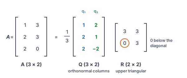
Find the QR factorization of A = \begin{bmatrix} 1 & 3 \\ 2 & 3 \\ 2 & 0 \end{bmatrix}.
v_1 = (1, 2, 2),\quad \|v_1\| = \sqrt{1 + 4 + 4} = 3First column and its length.
\frac{a_2 \cdot v_1}{v_1 \cdot v_1} = \frac{3 + 6 + 0}{9} = 1Weight of a₂ on v₁.
v_2 = (3 - 1, 3 - 2, 0 - 2) = (2, 1, -2),\quad \|v_2\| = \sqrt{4 + 1 + 4} = 3Subtract 1 times v₁, then find the length.
Q = \frac{1}{3}\begin{bmatrix} 1 & 2 \\ 2 & 1 \\ 2 & -2 \end{bmatrix}Divide both vectors by 3. Q is 3 × 2.
R = Q^T A = \frac{1}{3}\begin{bmatrix} 1 & 2 & 2 \\ 2 & 1 & -2 \end{bmatrix}\begin{bmatrix} 1 & 3 \\ 2 & 3 \\ 2 & 0 \end{bmatrix}Set up QᵀA. R is 2 × 2.
= \frac{1}{3}\begin{bmatrix} 1 + 4 + 4 & 3 + 6 + 0 \\ 2 + 2 - 4 & 6 + 3 - 0 \end{bmatrix} = \frac{1}{3}\begin{bmatrix} 9 & 9 \\ 0 & 9 \end{bmatrix} = \begin{bmatrix} 3 & 3 \\ 0 & 3 \end{bmatrix}Multiply, then multiply each entry by 1/3.
QR = \frac{1}{3}\begin{bmatrix} 3 + 0 & 3 + 6 \\ 6 + 0 & 6 + 3 \\ 6 + 0 & 6 - 6 \end{bmatrix} = \begin{bmatrix} 1 & 3 \\ 2 & 3 \\ 2 & 0 \end{bmatrix}Check: QR = A.
Answer: Q = \frac{1}{3}\begin{bmatrix} 1 & 2 \\ 2 & 1 \\ 2 & -2 \end{bmatrix} and R = \begin{bmatrix} 3 & 3 \\ 0 & 3 \end{bmatrix}.
Example 3: A 3 × 3 matrix
Find the QR factorization of A = \begin{bmatrix} 1 & 3 & 1 \\ 2 & 3 & 0 \\ 2 & 0 & 5 \end{bmatrix}. Its columns are the vectors from Example 3 of the Gram-Schmidt lesson.
v_1 = (1, 2, 2),\quad v_2 = (2, 1, -2),\quad v_3' = (2, -2, 1)
Gram-Schmidt on the columns, with v₃ scaled to clear fractions.
\|v_1\| = \|v_2\| = \|v_3'\| = 3
Each length is √9 = 3.
Q = \frac{1}{3}\begin{bmatrix} 1 & 2 & 2 \\ 2 & 1 & -2 \\ 2 & -2 & 1 \end{bmatrix}Divide each vector by 3. This square Q is an orthogonal matrix.
R = Q^T A = \frac{1}{3}\begin{bmatrix} 1 + 4 + 4 & 3 + 6 + 0 & 1 + 0 + 10 \\ 2 + 2 - 4 & 6 + 3 - 0 & 2 + 0 - 10 \\ 2 - 4 + 2 & 6 - 6 + 0 & 2 - 0 + 5 \end{bmatrix}Multiply Qᵀ by A. Here Qᵀ = Q because Q is symmetric.
= \frac{1}{3}\begin{bmatrix} 9 & 9 & 11 \\ 0 & 9 & -8 \\ 0 & 0 & 7 \end{bmatrix} = \begin{bmatrix} 3 & 3 & \tfrac{11}{3} \\ 0 & 3 & -\tfrac{8}{3} \\ 0 & 0 & \tfrac{7}{3} \end{bmatrix}Simplify. The zeros below the diagonal confirm the work.
\tfrac{11}{3}q_1 - \tfrac{8}{3}q_2 + \tfrac{7}{3}q_3 = \tfrac{1}{9}(11 - 16 + 14,\ 22 - 8 - 14,\ 22 + 16 + 7) = \tfrac{1}{9}(9, 0, 45) = (1, 0, 5)Check column 3 of QR against a₃.
Answer: Q = \frac{1}{3}\begin{bmatrix} 1 & 2 & 2 \\ 2 & 1 & -2 \\ 2 & -2 & 1 \end{bmatrix} and R = \begin{bmatrix} 3 & 3 & 11/3 \\ 0 & 3 & -8/3 \\ 0 & 0 & 7/3 \end{bmatrix}. The last diagonal entry, 7/3, is the length of the unscaled v₃ = (14/9, −14/9, 7/9).
Example 4: Solving Ax = b with QR
Use the QR factorization from Example 1 to solve Ax = b, where b = \begin{bmatrix} 1 \\ 18 \end{bmatrix}.
QRx = b \;\Rightarrow\; Rx = Q^T b
Multiply both sides by Qᵀ and use QᵀQ = I.
Q^T b = \frac{1}{5}\begin{bmatrix} 3(1) + 4(18) \\ -4(1) + 3(18) \end{bmatrix} = \frac{1}{5}\begin{bmatrix} 75 \\ 50 \end{bmatrix} = \begin{bmatrix} 15 \\ 10 \end{bmatrix}Multiply Qᵀ by b.
\begin{bmatrix} 5 & 10 \\ 0 & 5 \end{bmatrix}\begin{bmatrix} x_1 \\ x_2 \end{bmatrix} = \begin{bmatrix} 15 \\ 10 \end{bmatrix}Write the triangular system Rx = Qᵀb.
5x_2 = 10 \;\Rightarrow\; x_2 = 2
Solve the bottom row first (back substitution, as in Gaussian elimination).
5x_1 + 10(2) = 15
Substitute x₂ = 2 into the top row.
5x_1 = -5 \;\Rightarrow\; x_1 = -1
Subtract 20, then divide by 5.
A\begin{bmatrix} -1 \\ 2 \end{bmatrix} = \begin{bmatrix} -3 + 4 \\ -4 + 22 \end{bmatrix} = \begin{bmatrix} 1 \\ 18 \end{bmatrix}Check in the original system.
Answer: x = (−1, 2). No row reduction of A was needed, only one multiplication by Qᵀ and back substitution.
Example 5: Fitting a sales trend line with QR
A shop sold y = (10, 14, 15, 21) units in weeks t = 1, 2, 3, 4. The manager wants the line y = c + mt that fits best. The equations c + mt = y form the system Ax = y with A = \begin{bmatrix} 1 & 1 \\ 1 & 2 \\ 1 & 3 \\ 1 & 4 \end{bmatrix} and x = (c, m). No line passes through all four points, so solve Rx = Qᵀy, which gives the best fit.
v_1 = (1, 1, 1, 1),\quad \|v_1\| = 2,\quad q_1 = \tfrac{1}{2}(1, 1, 1, 1)First column, its length and q₁.
v_2 = (1, 2, 3, 4) - \tfrac{10}{4}(1, 1, 1, 1) = \left(-\tfrac{3}{2}, -\tfrac{1}{2}, \tfrac{1}{2}, \tfrac{3}{2}\right)Gram-Schmidt step with weight 10/4 = 5/2.
\|v_2\| = \sqrt{\tfrac{9}{4} + \tfrac{1}{4} + \tfrac{1}{4} + \tfrac{9}{4}} = \sqrt{5},\quad q_2 = \tfrac{1}{2\sqrt{5}}(-3, -1, 1, 3)Length of v₂, then divide by it.
r_{11} = 2,\quad r_{12} = q_1 \cdot a_2 = \tfrac{1 + 2 + 3 + 4}{2} = 5,\quad r_{22} = \sqrt{5}Entries of R.
q_1 \cdot y = \tfrac{10 + 14 + 15 + 21}{2} = \tfrac{60}{2} = 30First entry of Qᵀy.
q_2 \cdot y = \tfrac{-30 - 14 + 15 + 63}{2\sqrt{5}} = \tfrac{34}{2\sqrt{5}} = \tfrac{17}{\sqrt{5}}Second entry of Qᵀy.
\sqrt{5}\,m = \tfrac{17}{\sqrt{5}} \;\Rightarrow\; m = \tfrac{17}{5} = 3.4Bottom row of Rx = Qᵀy. Divide by √5.
2c + 5(3.4) = 30 \;\Rightarrow\; 2c = 13 \;\Rightarrow\; c = 6.5
Top row. Subtract 17, then divide by 2.
Answer: the best line is y = 6.5 + 3.4t, so sales grow by about 3.4 units a week, and the line predicts 6.5 + 3.4(5) = 23.5 units in week 5. This is the same line as the least-squares regression line for these data.
Common mistakes
| Mistake | Example of the error | Fix |
|---|---|---|
| Putting the unnormalized v’s in Q | Q = [3 −4; 4 3] in Example 1, so QᵀQ = 25I | Divide each vᵢ by its length so the columns of Q are unit vectors. |
| Multiplying in the wrong order | Finding R as AQᵀ or QAᵀ | R = QᵀA. Qᵀ goes on the left. |
| Making Q square when A is tall | Looking for a third column of Q in Example 2 | For a 3 × 2 matrix A, Q is 3 × 2 and R is 2 × 2. |
| Ignoring a nonzero entry below the diagonal | Getting r₂₁ = 1/5 and keeping it | r₂₁ = q₂ · a₁ must be 0. A nonzero value means a Gram-Schmidt or multiplication error. |
| Solving Rx = b instead of Rx = Qᵀb | In Example 4, getting x = (−7, 3.6), which gives Ax = (−13.8, 11.6) | Multiply b by Qᵀ first. Then back-substitute. |
Related ideas
QR compared with LU. LU decomposition splits A into triangular pieces using row operations. QR uses an orthonormal Q instead, which keeps rounding errors small, so software often prefers QR for least-squares problems.
Least squares. Example 5 is a preview. When Ax = b has no exact solution, Rx = Qᵀb gives the best approximate solution. Least-Squares Solutions explains why, using the normal equations.
Determinants. For a square A, the determinant of Q is 1 or −1, so |det A| is the product of the diagonal entries of R.
Eigenvalues. Repeating the steps “factor A = QR, then form RQ” gives the QR algorithm, which computers use to find eigenvalues of large matrices.
Practice problems
- Find the QR factorization of A = [1 4; 2 3].
- Find the QR factorization of the 3 × 2 matrix whose columns are (1, 0, 1) and (3, 2, 1).
- Check that QᵀQ = I for the matrix Q in Example 2.
- Q = [0.6 −0.8; 0.8 0.6] and R = [10 5; 0 5]. Find A = QR.
- Use your answer to Problem 1 to solve Ax = (3, 1).
- In any QR factorization, why is r₂₁ = q₂ · a₁ equal to 0?
- Find the QR factorization of the 3 × 2 matrix whose columns are (2, 1, 2) and (1, 1, 0).
- Find the QR factorization of A = [3 −4; 4 3], whose columns are already orthogonal.
- Use the QR factorization from Example 1 to find det A.
- Sales in weeks 1 to 4 were y = (8, 9, 13, 14). Use Q and R from Example 5 to find the best line y = c + mt.
Show answers
1.
v_1 = (1, 2),\quad v_2 = (4, 3) - 2(1, 2) = (2, -1)
Gram-Schmidt with weight (4 + 6)/5 = 2.
\|v_1\| = \|v_2\| = \sqrt{5},\quad Q = \tfrac{1}{\sqrt{5}}\begin{bmatrix} 1 & 2 \\ 2 & -1 \end{bmatrix}Normalize.
R = Q^T A = \tfrac{1}{\sqrt{5}}\begin{bmatrix} 1 + 4 & 4 + 6 \\ 2 - 2 & 8 - 3 \end{bmatrix} = \tfrac{1}{\sqrt{5}}\begin{bmatrix} 5 & 10 \\ 0 & 5 \end{bmatrix}Multiply Qᵀ by A.
= \begin{bmatrix} \sqrt{5} & 2\sqrt{5} \\ 0 & \sqrt{5} \end{bmatrix}5/√5 = √5 (see rationalizing the denominator).
Answer: Q = \tfrac{1}{\sqrt{5}}\begin{bmatrix} 1 & 2 \\ 2 & -1 \end{bmatrix}, R = \begin{bmatrix} \sqrt{5} & 2\sqrt{5} \\ 0 & \sqrt{5} \end{bmatrix}.
2.
v_1 = (1, 0, 1),\quad v_2 = (3, 2, 1) - 2(1, 0, 1) = (1, 2, -1)
Weight (3 + 1)/2 = 2.
\|v_1\| = \sqrt{2},\quad \|v_2\| = \sqrt{6}Lengths.
Q = \begin{bmatrix} 1/\sqrt{2} & 1/\sqrt{6} \\ 0 & 2/\sqrt{6} \\ 1/\sqrt{2} & -1/\sqrt{6} \end{bmatrix}Normalize the columns.
r_{11} = \sqrt{2},\quad r_{12} = \tfrac{3 + 0 + 1}{\sqrt{2}} = \tfrac{4}{\sqrt{2}} = 2\sqrt{2},\quad r_{22} = \tfrac{3 + 4 - 1}{\sqrt{6}} = \tfrac{6}{\sqrt{6}} = \sqrt{6}Entries of R = QᵀA (see simplifying square roots).
Answer: Q as above and R = \begin{bmatrix} \sqrt{2} & 2\sqrt{2} \\ 0 & \sqrt{6} \end{bmatrix}.
3.
Q^T Q = \tfrac{1}{9}\begin{bmatrix} 1 + 4 + 4 & 2 + 2 - 4 \\ 2 + 2 - 4 & 4 + 1 + 4 \end{bmatrix} = \tfrac{1}{9}\begin{bmatrix} 9 & 0 \\ 0 & 9 \end{bmatrix} = \begin{bmatrix} 1 & 0 \\ 0 & 1 \end{bmatrix}Dot products of the columns.
Answer: QᵀQ = I, so the columns of Q are orthonormal.
4.
QR = \begin{bmatrix} 0.6(10) + (-0.8)(0) & 0.6(5) + (-0.8)(5) \\ 0.8(10) + 0.6(0) & 0.8(5) + 0.6(5) \end{bmatrix}Multiply.
= \begin{bmatrix} 6 & 3 - 4 \\ 8 & 4 + 3 \end{bmatrix} = \begin{bmatrix} 6 & -1 \\ 8 & 7 \end{bmatrix}Simplify.
Answer: A = [6 −1; 8 7].
5.
Q^T b = \tfrac{1}{\sqrt{5}}(3 + 2,\ 6 - 1) = \tfrac{1}{\sqrt{5}}(5, 5) = (\sqrt{5}, \sqrt{5})Multiply Qᵀ by b = (3, 1).
\sqrt{5}\,x_2 = \sqrt{5} \;\Rightarrow\; x_2 = 1Bottom row of Rx = Qᵀb.
\sqrt{5}\,x_1 + 2\sqrt{5}(1) = \sqrt{5} \;\Rightarrow\; x_1 = -1Top row. Divide by √5, then subtract 2.
Answer: x = (−1, 1). Check: (−1 + 4, −2 + 3) = (3, 1).
6.
a_1 = r_{11}q_1Gram-Schmidt builds q₁ from a₁ alone, so a₁ is a multiple of q₁.
q_2 \cdot a_1 = r_{11}(q_2 \cdot q_1) = r_{11}(0) = 0q₂ is orthogonal to q₁.
Answer: r₂₁ = 0 because a₁ lies along q₁, and q₂ is orthogonal to q₁.
7.
v_1 = (2, 1, 2),\quad v_2' = (1, 2, -2),\quad \|v_1\| = \|v_2'\| = 3
Gram-Schmidt with weight 3/9 = 1/3, then multiply v₂ by 3.
Q = \tfrac{1}{3}\begin{bmatrix} 2 & 1 \\ 1 & 2 \\ 2 & -2 \end{bmatrix}Normalize.
R = Q^T A = \tfrac{1}{3}\begin{bmatrix} 4 + 1 + 4 & 2 + 1 + 0 \\ 2 + 2 - 4 & 1 + 2 + 0 \end{bmatrix} = \begin{bmatrix} 3 & 1 \\ 0 & 1 \end{bmatrix}Multiply and simplify.
Answer: Q = \tfrac{1}{3}\begin{bmatrix} 2 & 1 \\ 1 & 2 \\ 2 & -2 \end{bmatrix}, R = \begin{bmatrix} 3 & 1 \\ 0 & 1 \end{bmatrix}.
8.
(3, 4) \cdot (-4, 3) = -12 + 12 = 0
The columns are already orthogonal, so Gram-Schmidt changes nothing.
\|a_1\| = \|a_2\| = 5,\quad Q = \tfrac{1}{5}\begin{bmatrix} 3 & -4 \\ 4 & 3 \end{bmatrix}Normalize.
R = Q^T A = \tfrac{1}{5}\begin{bmatrix} 9 + 16 & -12 + 12 \\ -12 + 12 & 16 + 9 \end{bmatrix} = \begin{bmatrix} 5 & 0 \\ 0 & 5 \end{bmatrix}Multiply.
Answer: Q = A/5 and R = 5I.
9.
\det Q = \tfrac{9}{25} + \tfrac{16}{25} = 1,\quad \det R = 5 \cdot 5 = 25Determinant of each factor.
\det A = \det Q \cdot \det R = 1 \cdot 25 = 25
The determinant of a product is the product of the determinants.
Answer: det A = 25. Check: 3(11) − 2(4) = 33 − 8 = 25.
10.
q_1 \cdot y = \tfrac{8 + 9 + 13 + 14}{2} = 22,\quad q_2 \cdot y = \tfrac{-24 - 9 + 13 + 42}{2\sqrt{5}} = \tfrac{11}{\sqrt{5}}Compute Qᵀy.
\sqrt{5}\,m = \tfrac{11}{\sqrt{5}} \;\Rightarrow\; m = 2.2Bottom row.
2c + 5(2.2) = 22 \;\Rightarrow\; c = 5.5
Top row. Subtract 11, then divide by 2.
Answer: y = 5.5 + 2.2t.
QR factorization FAQ
What is QR factorization used for?
It is used to solve least-squares problems, to solve linear systems in a numerically stable way and, through the QR algorithm, to find eigenvalues.
How do you find R in a QR factorization?
After you build Q with the Gram-Schmidt process, multiply R = QᵀA. The diagonal entries are the lengths of the Gram-Schmidt vectors, and the entries below the diagonal are 0.
Does every matrix have a QR factorization?
Every matrix with linearly independent columns has one, with positive diagonal entries in R, and it is unique. Matrices with dependent columns also have QR factorizations, but they need methods beyond basic Gram-Schmidt.
What is the difference between QR and LU decomposition?
LU writes A as a lower triangular matrix times an upper triangular matrix using row operations. QR writes A as a matrix with orthonormal columns times an upper triangular matrix, and it works for tall matrices too.
Summary
- A = QR, where Q has orthonormal columns and R is upper triangular with a positive diagonal.
- Build Q with the Gram-Schmidt process on the columns of A, then normalize.
- Find R = QᵀA. Its diagonal holds the lengths ‖vᵢ‖, and its entries below the diagonal are 0.
- To solve Ax = b, solve the triangular system Rx = Qᵀb by back substitution.
- For a tall A, the same steps give the best-fit (least-squares) solution.
Previous lesson: Gram-Schmidt Process
Next lesson: Least-Squares Solutions
Back to the Linear Algebra Index