Orthogonal Diagonalization: Spectral Theorem

Orthogonal diagonalization writes a symmetric matrix as A = PDPᵀ, where D is diagonal and P is an orthogonal matrix whose columns are unit eigenvectors of A. The spectral theorem says this works for every symmetric matrix, and only for symmetric matrices. Because P⁻¹ = Pᵀ, you never have to compute an inverse.

Before this lesson: Diagonalization, Gram-Schmidt Process and Orthogonal Sets and Orthonormal Bases

Why symmetric matrices are special

A matrix is symmetric when Aᵀ = A, so its entries mirror across the main diagonal (see transpose of a matrix). Symmetric matrices show up everywhere: distances, covariances, stresses and quadratic forms all produce them.

Ordinary diagonalization needs n independent eigenvectors, and they can point in any directions. A symmetric matrix does better. Its eigenvalues are real, and it has n eigenvectors that are perpendicular to each other. So the matrix just stretches space along perpendicular axes.

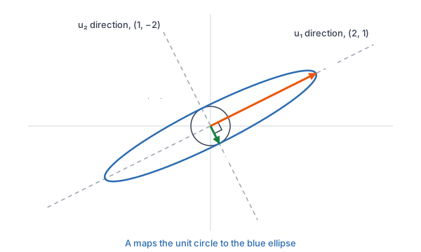
The unit circle and its image under the symmetric matrix A = [5 2; 2 2], an ellipse centered at the origin. The long axis of the ellipse lies along the eigenvector direction u1 = (2, 1)/√5 and is stretched by 6. The short axis lies along the perpendicular direction u2 = (1, −2)/√5 and is stretched by 1. Dashed lines show the two perpendicular eigenvector directions. — A symmetric matrix stretches along perpendicular eigenvector directions: by 6 along u₁ and by 1 along u₂.

The spectral theorem

An n × n matrix A is orthogonally diagonalizable if A = PDPᵀ for an orthogonal matrix P (PᵀP = I) and a diagonal matrix D.

A \text{ is orthogonally diagonalizable} \iff A^T = A

Every eigenvalue of a symmetric matrix is a real number.
Eigenvectors from different eigenvalues are automatically orthogonal.
For a repeated eigenvalue, the eigenspace has dimension equal to the number of times the eigenvalue repeats. Use the Gram-Schmidt process inside that eigenspace to get orthogonal vectors.
Spectral decomposition: if P has columns u₁, …, uₙ with eigenvalues λ₁, …, λₙ, then A = λ₁u₁u₁ᵀ + … + λₙuₙuₙᵀ. Each uᵢuᵢᵀ is the projection matrix onto the line through uᵢ.

How to orthogonally diagonalize a matrix

Check that A is symmetric. If it is not, it cannot be orthogonally diagonalized.
Find the eigenvalues from det(A − λI) = 0.
Find a basis for each eigenspace. For a repeated eigenvalue, make that basis orthogonal with Gram-Schmidt.
Divide every eigenvector by its length. These unit vectors are the columns of P.
Put the matching eigenvalues on the diagonal of D, in the same order as the columns of P. Check that PDPᵀ = A.

Orthogonal diagonalization examples

Example 1: A 2 × 2 symmetric matrix

Orthogonally diagonalize $A = \begin{bmatrix} 5 & 2 \\ 2 & 2 \end{bmatrix}$ .

\det(A - \lambda I) = (5 - \lambda)(2 - \lambda) - 2 \cdot 2 = \lambda^2 - 7\lambda + 6

Aᵀ = A. Find the characteristic polynomial.

\lambda^2 - 7\lambda + 6 = (\lambda - 6)(\lambda - 1) = 0 \;\Rightarrow\; \lambda = 6,\ 1

Factor (see factoring trinomials).

A - 6I = \begin{bmatrix} -1 & 2 \\ 2 & -4 \end{bmatrix} \;\Rightarrow\; -x + 2y = 0 \;\Rightarrow\; v_1 = \begin{bmatrix} 2 \\ 1 \end{bmatrix}

Eigenvector for λ = 6 (see eigenvalues and eigenvectors).

A - I = \begin{bmatrix} 4 & 2 \\ 2 & 1 \end{bmatrix} \;\Rightarrow\; 2x + y = 0 \;\Rightarrow\; v_2 = \begin{bmatrix} 1 \\ -2 \end{bmatrix}

Eigenvector for λ = 1.

v_1 \cdot v_2 = 2 - 2 = 0

Check: the eigenvectors are orthogonal, as the theorem promises.

\|v_1\| = \|v_2\| = \sqrt{5}

Both lengths are √(4 + 1).

P = \frac{1}{\sqrt{5}}\begin{bmatrix} 2 & 1 \\ 1 & -2 \end{bmatrix},\quad D = \begin{bmatrix} 6 & 0 \\ 0 & 1 \end{bmatrix}

Unit eigenvectors as columns, eigenvalues in the same order.

PDP^T = \frac{1}{5}\begin{bmatrix} 12 & 1 \\ 6 & -2 \end{bmatrix}\begin{bmatrix} 2 & 1 \\ 1 & -2 \end{bmatrix}

First multiply P by D, which scales column 1 by 6 (see matrix multiplication).

= \frac{1}{5}\begin{bmatrix} 24 + 1 & 12 - 2 \\ 12 - 2 & 6 + 4 \end{bmatrix} = \frac{1}{5}\begin{bmatrix} 25 & 10 \\ 10 & 10 \end{bmatrix} = \begin{bmatrix} 5 & 2 \\ 2 & 2 \end{bmatrix}

Multiply by Pᵀ and simplify. This equals A.

Answer: $A = PDP^T$ with $P = \frac{1}{\sqrt{5}}\begin{bmatrix} 2 & 1 \\ 1 & -2 \end{bmatrix}$ and $D = \begin{bmatrix} 6 & 0 \\ 0 & 1 \end{bmatrix}$ .

Example 2: A 3 × 3 matrix with three different eigenvalues

Orthogonally diagonalize $A = \begin{bmatrix} 1 & -1 & 0 \\ -1 & 2 & -1 \\ 0 & -1 & 1 \end{bmatrix}$ . Its characteristic polynomial is det(A − λI) = −λ(λ − 1)(λ − 3), so the eigenvalues are 3, 1 and 0.

A - 3I = \begin{bmatrix} -2 & -1 & 0 \\ -1 & -1 & -1 \\ 0 & -1 & -2 \end{bmatrix}

Start with λ = 3.

y = -2x,\quad y = -2z \;\Rightarrow\; v_1 = (1, -2, 1)

Rows 1 and 3 give y in terms of x and z, so z = x. Row 2 checks: −1 + 2 − 1 = 0.

A - I = \begin{bmatrix} 0 & -1 & 0 \\ -1 & 1 & -1 \\ 0 & -1 & 0 \end{bmatrix} \;\Rightarrow\; y = 0,\ x = -z \;\Rightarrow\; v_2 = (1, 0, -1)

λ = 1: row 1 gives y = 0, then row 2 gives −x − z = 0.

A - 0I = A \;\Rightarrow\; x = y,\ z = y \;\Rightarrow\; v_3 = (1, 1, 1)

λ = 0: rows 1 and 3 give x − y = 0 and z − y = 0.

v_1 \cdot v_2 = 1 + 0 - 1 = 0,\quad v_1 \cdot v_3 = 1 - 2 + 1 = 0,\quad v_2 \cdot v_3 = 1 + 0 - 1 = 0

Check: all three pairs are orthogonal.

\|v_1\| = \sqrt{6},\quad \|v_2\| = \sqrt{2},\quad \|v_3\| = \sqrt{3}

Lengths.

P = \begin{bmatrix} 1/\sqrt{6} & 1/\sqrt{2} & 1/\sqrt{3} \\ -2/\sqrt{6} & 0 & 1/\sqrt{3} \\ 1/\sqrt{6} & -1/\sqrt{2} & 1/\sqrt{3} \end{bmatrix},\quad D = \begin{bmatrix} 3 & 0 & 0 \\ 0 & 1 & 0 \\ 0 & 0 & 0 \end{bmatrix}

Unit eigenvectors as columns.

Answer: A = PDPᵀ with P and D above. Distinct eigenvalues gave orthogonal eigenvectors with no extra work.

Example 3: A repeated eigenvalue

Orthogonally diagonalize $A = \begin{bmatrix} 2 & 1 & 1 \\ 1 & 2 & 1 \\ 1 & 1 & 2 \end{bmatrix}$ , whose eigenvalues are 4, 1 and 1.

A\begin{bmatrix} 1 \\ 1 \\ 1 \end{bmatrix} = \begin{bmatrix} 2 + 1 + 1 \\ 1 + 2 + 1 \\ 1 + 1 + 2 \end{bmatrix} = 4\begin{bmatrix} 1 \\ 1 \\ 1 \end{bmatrix}

Each row adds to 4, so v₁ = (1, 1, 1) is an eigenvector for λ = 4.

A - I = \begin{bmatrix} 1 & 1 & 1 \\ 1 & 1 & 1 \\ 1 & 1 & 1 \end{bmatrix} \;\Rightarrow\; x + y + z = 0

λ = 1: every row gives the same equation, so the eigenspace is a plane.

x_1 = (-1, 1, 0),\quad x_2 = (-1, 0, 1)

A basis for the plane, from parametric vector form with y and z free.

x_1 \cdot x_2 = 1 + 0 + 0 = 1 \ne 0

This basis is not orthogonal, so apply Gram-Schmidt.

v_3 = x_2 - \frac{x_2 \cdot x_1}{x_1 \cdot x_1}x_1 = (-1, 0, 1) - \tfrac{1}{2}(-1, 1, 0) = \left(-\tfrac{1}{2}, -\tfrac{1}{2}, 1\right)

Subtract the projection onto x₁.

v_2 = x_1 = (-1, 1, 0),\quad v_3' = 2v_3 = (-1, -1, 2)

Keep x₁ and clear fractions in v₃.

v_1 \cdot v_2 = 0,\quad v_1 \cdot v_3' = -1 - 1 + 2 = 0,\quad v_2 \cdot v_3' = 1 - 1 + 0 = 0

Check all three pairs. The first is −1 + 1 + 0 = 0.

P = \begin{bmatrix} 1/\sqrt{3} & -1/\sqrt{2} & -1/\sqrt{6} \\ 1/\sqrt{3} & 1/\sqrt{2} & -1/\sqrt{6} \\ 1/\sqrt{3} & 0 & 2/\sqrt{6} \end{bmatrix},\quad D = \begin{bmatrix} 4 & 0 & 0 \\ 0 & 1 & 0 \\ 0 & 0 & 1 \end{bmatrix}

Normalize: the lengths are √3, √2 and √6.

Answer: A = PDPᵀ with P and D above. Without the Gram-Schmidt step, the two columns for λ = 1 would not be orthogonal and P would not be an orthogonal matrix.

Example 4: The spectral decomposition

Write A from Example 1 as a sum λ₁u₁u₁ᵀ + λ₂u₂u₂ᵀ.

u_1 u_1^T = \frac{1}{5}\begin{bmatrix} 2 \\ 1 \end{bmatrix}\begin{bmatrix} 2 & 1 \end{bmatrix} = \frac{1}{5}\begin{bmatrix} 4 & 2 \\ 2 & 1 \end{bmatrix}

Column times row, with u₁ = (2, 1)/√5.

u_2 u_2^T = \frac{1}{5}\begin{bmatrix} 1 \\ -2 \end{bmatrix}\begin{bmatrix} 1 & -2 \end{bmatrix} = \frac{1}{5}\begin{bmatrix} 1 & -2 \\ -2 & 4 \end{bmatrix}

Same for u₂ = (1, −2)/√5.

6u_1u_1^T + 1u_2u_2^T = \frac{1}{5}\begin{bmatrix} 24 + 1 & 12 - 2 \\ 12 - 2 & 6 + 4 \end{bmatrix}

Multiply by the eigenvalues and add.

= \frac{1}{5}\begin{bmatrix} 25 & 10 \\ 10 & 10 \end{bmatrix} = \begin{bmatrix} 5 & 2 \\ 2 & 2 \end{bmatrix}

Simplify. This is A.

Answer: A = 6u₁u₁ᵀ + u₂u₂ᵀ. Each piece is an eigenvalue times the projection matrix onto one eigenvector direction.

Example 5: Principal stresses in a steel plate

An engineer measures the stress at one point of a steel plate as the symmetric matrix $S = \begin{bmatrix} 80 & 30 \\ 30 & 0 \end{bmatrix}$ (in MPa). The eigenvalues are the principal stresses, and the unit eigenvectors are the directions in which they act. Find both.

\det(S - \lambda I) = (80 - \lambda)(-\lambda) - 900 = \lambda^2 - 80\lambda - 900

Characteristic polynomial.

\lambda^2 - 80\lambda - 900 = (\lambda - 90)(\lambda + 10) = 0 \;\Rightarrow\; \lambda = 90,\ -10

Factor: −90 · 10 = −900 and −90 + 10 = −80.

S - 90I = \begin{bmatrix} -10 & 30 \\ 30 & -90 \end{bmatrix} \;\Rightarrow\; x = 3y \;\Rightarrow\; u_1 = \tfrac{1}{\sqrt{10}}(3, 1)

Direction for λ = 90, normalized by √(9 + 1).

S + 10I = \begin{bmatrix} 90 & 30 \\ 30 & 10 \end{bmatrix} \;\Rightarrow\; y = -3x \;\Rightarrow\; u_2 = \tfrac{1}{\sqrt{10}}(1, -3)

Direction for λ = −10.

u_1 \cdot u_2 = \tfrac{3 - 3}{10} = 0

The two directions are perpendicular.

\theta = \tan^{-1}\!\left(\tfrac{1}{3}\right) \approx 18.4^\circ

Angle of u₁ from the x-axis (see inverse trig functions).

Answer: the plate feels a maximum tension of 90 MPa along the direction about 18.4° above the x-axis and a compression of 10 MPa along the perpendicular direction. In the u₁u₂ axes the stress matrix is simply D = [90 0; 0 −10].

Common mistakes

Mistake	Example of the error	Fix
Forgetting to normalize the columns of P	Using P = [2 1; 1 −2] in Example 1, so PᵀP = 5I	Divide each eigenvector by its length so that PᵀP = I.
Keeping a non-orthogonal basis for a repeated eigenvalue	Using (−1, 1, 0) and (−1, 0, 1) in Example 3, whose dot product is 1	Apply Gram-Schmidt inside the eigenspace.
Trying it on a matrix that is not symmetric	Looking for orthogonal eigenvectors of [1 2; 0 3]	Its eigenvectors (1, 0) and (1, 1) are not orthogonal. Only symmetric matrices are orthogonally diagonalizable.
Listing the eigenvalues in the wrong order	P from Example 1 with D = [1 0; 0 6] gives [2 −2; −2 5], not A	Column i of P must go with diagonal entry i of D.
Computing P⁻¹ the long way	Row reducing [P \| I] for a 3 × 3 P	For an orthogonal matrix, P⁻¹ = Pᵀ. Just transpose.

Related ideas

Quadratic forms. An expression like 5x² + 4xy + 2y² equals xᵀAx with A from Example 1. In the eigenvector coordinates it becomes 6X² + Y², with no cross term. This is how rotated ellipses and hyperbolas are put in standard position, so they can be named as in identifying conic sections.

Positive definite matrices. A symmetric matrix with all eigenvalues positive is called positive definite. Then xᵀAx is positive for every nonzero x, which is what the second derivative test for extrema of functions of two variables checks.

Every matrix. Non-symmetric and even non-square matrices have a similar factorization with two different orthogonal matrices. The next lesson, Singular Value Decomposition, builds it from the orthogonal diagonalization of AᵀA.

Practice problems

Orthogonally diagonalize A = [3 1; 1 3].
Orthogonally diagonalize A = [2 −2; −2 5].
Can A = [1 2; 0 3] be orthogonally diagonalized? Explain.
Orthogonally diagonalize A = [4 3; 3 −4].
Write the spectral decomposition of A = [3 1; 1 3] from Problem 1.
Orthogonally diagonalize A = [2 0 0; 0 3 1; 0 1 3].
Use A = PDPᵀ from Example 1 to find A⁵.
Show that if A is symmetric, Av₁ = λ₁v₁ and Av₂ = λ₂v₂ with λ₁ ≠ λ₂, then v₁ · v₂ = 0.
Use Problem 1 to write 3x² + 2xy + 3y² = 8 with no xy term, and name the curve.
A stress matrix is S = [10 6; 6 −6] (MPa). Find the principal stresses and their directions.

Show answers

\lambda^2 - 6\lambda + 8 = (\lambda - 4)(\lambda - 2)

Characteristic polynomial: (3 − λ)² − 1.

\lambda = 4:\ v_1 = (1, 1),\qquad \lambda = 2:\ v_2 = (1, -1)

A − 4I gives −x + y = 0. A − 2I gives x + y = 0.

P = \tfrac{1}{\sqrt{2}}\begin{bmatrix} 1 & 1 \\ 1 & -1 \end{bmatrix},\quad D = \begin{bmatrix} 4 & 0 \\ 0 & 2 \end{bmatrix}

Normalize by √2.

Answer: A = PDPᵀ with P and D above.

\lambda^2 - 7\lambda + 6 = (\lambda - 6)(\lambda - 1)

(2 − λ)(5 − λ) − 4.

\lambda = 6:\ v_1 = (1, -2),\qquad \lambda = 1:\ v_2 = (2, 1)

A − 6I gives −4x − 2y = 0. A − I gives x − 2y = 0.

P = \tfrac{1}{\sqrt{5}}\begin{bmatrix} 1 & 2 \\ -2 & 1 \end{bmatrix},\quad D = \begin{bmatrix} 6 & 0 \\ 0 & 1 \end{bmatrix}

Normalize by √5.

Answer: A = PDPᵀ with P and D above.

A^T = \begin{bmatrix} 1 & 0 \\ 2 & 3 \end{bmatrix} \ne A

A is not symmetric.

(1, 0) \cdot (1, 1) = 1 \ne 0

Its eigenvectors for λ = 1 and λ = 3 are not orthogonal.

Answer: no. A is diagonalizable, but not with an orthogonal P.

\lambda^2 - 25 = 0 \;\Rightarrow\; \lambda = 5,\ -5

(4 − λ)(−4 − λ) − 9 = λ² − 16 − 9.

\lambda = 5:\ v_1 = (3, 1),\qquad \lambda = -5:\ v_2 = (1, -3)

A − 5I gives −x + 3y = 0. A + 5I gives 3x + y = 0.

P = \tfrac{1}{\sqrt{10}}\begin{bmatrix} 3 & 1 \\ 1 & -3 \end{bmatrix},\quad D = \begin{bmatrix} 5 & 0 \\ 0 & -5 \end{bmatrix}

Normalize by √10.

Answer: A = PDPᵀ with P and D above.

4 \cdot \tfrac{1}{2}\begin{bmatrix} 1 & 1 \\ 1 & 1 \end{bmatrix} + 2 \cdot \tfrac{1}{2}\begin{bmatrix} 1 & -1 \\ -1 & 1 \end{bmatrix}

u₁u₁ᵀ and u₂u₂ᵀ with u₁ = (1, 1)/√2 and u₂ = (1, −1)/√2.

= \begin{bmatrix} 2 + 1 & 2 - 1 \\ 2 - 1 & 2 + 1 \end{bmatrix} = \begin{bmatrix} 3 & 1 \\ 1 & 3 \end{bmatrix}

Add. This is A.

Answer: A = 4u₁u₁ᵀ + 2u₂u₂ᵀ.

\lambda = 2:\ x \text{ free},\ y + z = 0 \;\Rightarrow\; (1, 0, 0),\ (0, 1, -1)

A − 2I has rows (0, 0, 0), (0, 1, 1), (0, 1, 1). These two vectors are already orthogonal.

\lambda = 4:\ (0, 1, 1)

A − 4I gives x = 0 and y = z.

P = \begin{bmatrix} 1 & 0 & 0 \\ 0 & 1/\sqrt{2} & 1/\sqrt{2} \\ 0 & -1/\sqrt{2} & 1/\sqrt{2} \end{bmatrix},\quad D = \begin{bmatrix} 2 & 0 & 0 \\ 0 & 2 & 0 \\ 0 & 0 & 4 \end{bmatrix}

Normalize.

Answer: A = PDPᵀ with P and D above.

A^5 = PD^5P^T = 6^5 u_1u_1^T + 1^5 u_2u_2^T

The PᵀP factors in the middle cancel.

= \tfrac{7776}{5}\begin{bmatrix} 4 & 2 \\ 2 & 1 \end{bmatrix} + \tfrac{1}{5}\begin{bmatrix} 1 & -2 \\ -2 & 4 \end{bmatrix}

Use the pieces from Example 4.

= \tfrac{1}{5}\begin{bmatrix} 31105 & 15550 \\ 15550 & 7780 \end{bmatrix} = \begin{bmatrix} 6221 & 3110 \\ 3110 & 1556 \end{bmatrix}

Add, then divide by 5.

Answer: A⁵ = [6221 3110; 3110 1556].

\lambda_1(v_1 \cdot v_2) = (Av_1) \cdot v_2 = v_1 \cdot (A^T v_2)

Move A across the dot product with a transpose.

= v_1 \cdot (Av_2) = \lambda_2(v_1 \cdot v_2)

Aᵀ = A because A is symmetric.

(\lambda_1 - \lambda_2)(v_1 \cdot v_2) = 0

Subtract.

Answer: λ₁ − λ₂ ≠ 0, so v₁ · v₂ = 0.

3x^2 + 2xy + 3y^2 = x^T\begin{bmatrix} 3 & 1 \\ 1 & 3 \end{bmatrix}x

Half of the xy coefficient goes in each off-diagonal spot.

4X^2 + 2Y^2 = 8 \;\Rightarrow\; \frac{X^2}{2} + \frac{Y^2}{4} = 1

Use the eigenvalues 4 and 2, then divide by 8.

Answer: an ellipse, with semi-axis √2 along (1, 1) and semi-axis 2 along (1, −1).

10.

\lambda^2 - 4\lambda - 96 = (\lambda - 12)(\lambda + 8)

(10 − λ)(−6 − λ) − 36 = λ² − 4λ − 60 − 36.

\lambda = 12:\ (3, 1),\qquad \lambda = -8:\ (1, -3)

S − 12I gives −2x + 6y = 0. S + 8I gives 18x + 6y = 0.

Answer: principal stresses 12 MPa along (3, 1)/√10 and −8 MPa along (1, −3)/√10.

Orthogonal diagonalization FAQ

Which matrices can be orthogonally diagonalized?

Exactly the symmetric matrices. This is the spectral theorem.

What is the difference between diagonalization and orthogonal diagonalization?

Diagonalization writes A = PDP⁻¹ with any invertible P. Orthogonal diagonalization requires P to be orthogonal, so A = PDPᵀ, and that is possible only for symmetric matrices.

Are the eigenvectors of a symmetric matrix always orthogonal?

Eigenvectors for different eigenvalues always are. Within the eigenspace of a repeated eigenvalue you can choose them orthogonal, using Gram-Schmidt.

What is the spectral theorem used for?

It explains principal axes of ellipses, principal stresses, principal component analysis in statistics and the singular value decomposition.

Summary

A matrix is orthogonally diagonalizable, A = PDPᵀ, exactly when it is symmetric.
Its eigenvalues are real, and eigenvectors for different eigenvalues are orthogonal.
Use Gram-Schmidt inside the eigenspace of a repeated eigenvalue.
Normalize the eigenvectors to build P, and keep D in the same order.
Spectral decomposition: A = λ₁u₁u₁ᵀ + … + λₙuₙuₙᵀ.

Previous lesson: Least-Squares Solutions

Next lesson: Singular Value Decomposition

Back to the Linear Algebra Index