
Singular Value Decomposition
The singular value decomposition (SVD) factors any m × n matrix as A = UΣVᵀ. U and V are orthogonal matrices, and Σ is diagonal with the singular values σ₁ ≥ σ₂ ≥ … ≥ 0. The singular values are the square roots of the eigenvalues of AᵀA, and they measure how much A stretches space.
Before this lesson: Orthogonal Diagonalization, Eigenvalues and Eigenvectors and Rank of a Matrix
What the SVD tells you
Only symmetric matrices can be orthogonally diagonalized. The SVD gets almost the same result for every matrix, square or not, by using two different orthonormal bases: one for the inputs and one for the outputs.
Picture A acting on the unit circle. It turns the circle into an ellipse. The perpendicular input directions v₁ and v₂ that land on the ellipse’s axes are the columns of V. The axis directions u₁ and u₂ are the columns of U, and the axis lengths are the singular values.
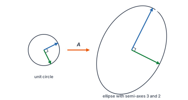
The singular value decomposition
Every m × n matrix A can be written as
A = U\Sigma V^T
- V is n × n and orthogonal. Its columns vᵢ are orthonormal eigenvectors of the symmetric matrix AᵀA, found by orthogonal diagonalization.
- Σ is m × n with the singular values σᵢ = √λᵢ on its diagonal, from largest to smallest, and zeros everywhere else. Here λᵢ are the eigenvalues of AᵀA, which are never negative.
- U is m × m and orthogonal. For each σᵢ > 0, its column is uᵢ = Avᵢ/σᵢ. Any remaining columns complete an orthonormal basis of ℝᵐ.
- The rank of A equals the number of nonzero singular values.
- Outer product form: A = σ₁u₁v₁ᵀ + σ₂u₂v₂ᵀ + … + σᵣuᵣvᵣᵀ, where r is the rank.
How to find the SVD
- Compute AᵀA.
- Find its eigenvalues, list them from largest to smallest, and take square roots to get the singular values.
- Find orthonormal eigenvectors vᵢ of AᵀA, in the same order. They are the columns of V.
- For each nonzero σᵢ, compute uᵢ = Avᵢ/σᵢ. If U needs more columns, add unit vectors orthogonal to the ones you have.
- Build Σ the same size as A, and check that UΣVᵀ = A.
Singular value decomposition examples
Example 1: A 2 × 2 matrix
Find the SVD of A = \begin{bmatrix} 2 & -1 \\ 2 & 2 \end{bmatrix}.
A^T A = \begin{bmatrix} 2 & 2 \\ -1 & 2 \end{bmatrix}\begin{bmatrix} 2 & -1 \\ 2 & 2 \end{bmatrix} = \begin{bmatrix} 4 + 4 & -2 + 4 \\ -2 + 4 & 1 + 4 \end{bmatrix} = \begin{bmatrix} 8 & 2 \\ 2 & 5 \end{bmatrix}Multiply Aᵀ by A (see transpose of a matrix).
(8 - \lambda)(5 - \lambda) - 4 = \lambda^2 - 13\lambda + 36 = (\lambda - 9)(\lambda - 4)
Characteristic polynomial of AᵀA, then factor.
\sigma_1 = \sqrt{9} = 3,\quad \sigma_2 = \sqrt{4} = 2Singular values, largest first.
A^T A - 9I = \begin{bmatrix} -1 & 2 \\ 2 & -4 \end{bmatrix} \;\Rightarrow\; x = 2y \;\Rightarrow\; v_1 = \tfrac{1}{\sqrt{5}}(2, 1)Unit eigenvector for λ = 9.
A^T A - 4I = \begin{bmatrix} 4 & 2 \\ 2 & 1 \end{bmatrix} \;\Rightarrow\; y = -2x \;\Rightarrow\; v_2 = \tfrac{1}{\sqrt{5}}(1, -2)Unit eigenvector for λ = 4.
u_1 = \frac{Av_1}{\sigma_1} = \frac{1}{3\sqrt{5}}(4 - 1,\ 4 + 2) = \frac{1}{3\sqrt{5}}(3, 6) = \tfrac{1}{\sqrt{5}}(1, 2)Multiply A by v₁, then divide by 3.
u_2 = \frac{Av_2}{\sigma_2} = \frac{1}{2\sqrt{5}}(2 + 2,\ 2 - 4) = \frac{1}{2\sqrt{5}}(4, -2) = \tfrac{1}{\sqrt{5}}(2, -1)Multiply A by v₂, then divide by 2.
U\Sigma V^T = \frac{1}{5}\begin{bmatrix} 1 & 2 \\ 2 & -1 \end{bmatrix}\begin{bmatrix} 3 & 0 \\ 0 & 2 \end{bmatrix}\begin{bmatrix} 2 & 1 \\ 1 & -2 \end{bmatrix}Set up the check. The two factors of 1/√5 make 1/5.
= \frac{1}{5}\begin{bmatrix} 3 & 4 \\ 6 & -2 \end{bmatrix}\begin{bmatrix} 2 & 1 \\ 1 & -2 \end{bmatrix} = \frac{1}{5}\begin{bmatrix} 6 + 4 & 3 - 8 \\ 12 - 2 & 6 + 4 \end{bmatrix} = \begin{bmatrix} 2 & -1 \\ 2 & 2 \end{bmatrix}Multiply left to right (see matrix multiplication). This is A.
Answer: U = \tfrac{1}{\sqrt{5}}\begin{bmatrix} 1 & 2 \\ 2 & -1 \end{bmatrix}, \Sigma = \begin{bmatrix} 3 & 0 \\ 0 & 2 \end{bmatrix} and V = \tfrac{1}{\sqrt{5}}\begin{bmatrix} 2 & 1 \\ 1 & -2 \end{bmatrix}.
Example 2: A tall 3 × 2 matrix
Find the SVD of A = \begin{bmatrix} 1 & 1 \\ 0 & 1 \\ 1 & 0 \end{bmatrix}.
A^T A = \begin{bmatrix} 1 + 0 + 1 & 1 + 0 + 0 \\ 1 + 0 + 0 & 1 + 1 + 0 \end{bmatrix} = \begin{bmatrix} 2 & 1 \\ 1 & 2 \end{bmatrix}AᵀA is 2 × 2.
(2 - \lambda)^2 - 1 = (\lambda - 3)(\lambda - 1) \;\Rightarrow\; \sigma_1 = \sqrt{3},\ \sigma_2 = 1Eigenvalues 3 and 1, then square roots.
v_1 = \tfrac{1}{\sqrt{2}}(1, 1),\quad v_2 = \tfrac{1}{\sqrt{2}}(1, -1)Unit eigenvectors for λ = 3 and λ = 1.
u_1 = \frac{Av_1}{\sqrt{3}} = \frac{1}{\sqrt{3}} \cdot \frac{1}{\sqrt{2}}(2, 1, 1) = \tfrac{1}{\sqrt{6}}(2, 1, 1)Av₁ adds the two columns.
u_2 = \frac{Av_2}{1} = \tfrac{1}{\sqrt{2}}(0, -1, 1)Av₂ subtracts column 2 from column 1.
(2, 1, 1) \times (0, -1, 1) = (1 + 1,\ 0 - 2,\ -2 - 0) = (2, -2, -2) \;\Rightarrow\; u_3 = \tfrac{1}{\sqrt{3}}(1, -1, -1)U needs a third column orthogonal to u₁ and u₂. Use the cross product, then normalize.
\Sigma = \begin{bmatrix} \sqrt{3} & 0 \\ 0 & 1 \\ 0 & 0 \end{bmatrix}Σ has the same size as A, 3 × 2.
Answer: U = \begin{bmatrix} 2/\sqrt{6} & 0 & 1/\sqrt{3} \\ 1/\sqrt{6} & -1/\sqrt{2} & -1/\sqrt{3} \\ 1/\sqrt{6} & 1/\sqrt{2} & -1/\sqrt{3} \end{bmatrix}, Σ as above and V = \tfrac{1}{\sqrt{2}}\begin{bmatrix} 1 & 1 \\ 1 & -1 \end{bmatrix}. The third column of U meets a row of zeros in Σ, so the short form A = σ₁u₁v₁ᵀ + σ₂u₂v₂ᵀ does not need it.
Example 3: A matrix of rank 1
Find the SVD of A = \begin{bmatrix} 2 & 4 \\ 1 & 2 \end{bmatrix} and its rank.
A^T A = \begin{bmatrix} 4 + 1 & 8 + 2 \\ 8 + 2 & 16 + 4 \end{bmatrix} = \begin{bmatrix} 5 & 10 \\ 10 & 20 \end{bmatrix}Multiply Aᵀ by A.
(5 - \lambda)(20 - \lambda) - 100 = \lambda^2 - 25\lambda = \lambda(\lambda - 25)
The constant terms cancel: 100 − 100 = 0.
\sigma_1 = 5,\quad \sigma_2 = 0
Square roots of 25 and 0.
v_1 = \tfrac{1}{\sqrt{5}}(1, 2),\quad v_2 = \tfrac{1}{\sqrt{5}}(2, -1)AᵀA − 25I gives y = 2x. v₂ is the perpendicular unit vector.
u_1 = \frac{Av_1}{5} = \frac{1}{5\sqrt{5}}(2 + 8,\ 1 + 4) = \tfrac{1}{\sqrt{5}}(2, 1)Divide (10, 5)/√5 by 5.
u_2 = \tfrac{1}{\sqrt{5}}(1, -2)σ₂ = 0, so u₂ cannot come from Av₂/σ₂. Take the unit vector orthogonal to u₁.
\sigma_1 u_1 v_1^T = 5 \cdot \tfrac{1}{5}\begin{bmatrix} 2 \\ 1 \end{bmatrix}\begin{bmatrix} 1 & 2 \end{bmatrix} = \begin{bmatrix} 2 & 4 \\ 1 & 2 \end{bmatrix}Check with the outer product form. One term already gives A.
Answer: σ₁ = 5, σ₂ = 0, U = \tfrac{1}{\sqrt{5}}\begin{bmatrix} 2 & 1 \\ 1 & -2 \end{bmatrix} and V = \tfrac{1}{\sqrt{5}}\begin{bmatrix} 1 & 2 \\ 2 & -1 \end{bmatrix}. One nonzero singular value means rank A = 1.
Example 4: The best rank-1 approximation
Use the SVD from Example 1 to find the rank-1 matrix closest to A, and the size of the error.
A_1 = \sigma_1 u_1 v_1^T = 3 \cdot \tfrac{1}{5}\begin{bmatrix} 1 \\ 2 \end{bmatrix}\begin{bmatrix} 2 & 1 \end{bmatrix} = \tfrac{3}{5}\begin{bmatrix} 2 & 1 \\ 4 & 2 \end{bmatrix} = \begin{bmatrix} 1.2 & 0.6 \\ 2.4 & 1.2 \end{bmatrix}Keep only the largest term of the outer product form.
A - A_1 = \begin{bmatrix} 2 - 1.2 & -1 - 0.6 \\ 2 - 2.4 & 2 - 1.2 \end{bmatrix} = \begin{bmatrix} 0.8 & -1.6 \\ -0.4 & 0.8 \end{bmatrix}The part that was left out.
\sigma_2 u_2 v_2^T = 2 \cdot \tfrac{1}{5}\begin{bmatrix} 2 \\ -1 \end{bmatrix}\begin{bmatrix} 1 & -2 \end{bmatrix} = \tfrac{2}{5}\begin{bmatrix} 2 & -4 \\ -1 & 2 \end{bmatrix} = \begin{bmatrix} 0.8 & -1.6 \\ -0.4 & 0.8 \end{bmatrix}Check: the leftover is exactly the second term.
\sqrt{0.64 + 2.56 + 0.16 + 0.64} = \sqrt{4} = 2 = \sigma_2Size of the error (square root of the sum of squared entries).
Answer: A₁ = [1.2 0.6; 2.4 1.2], and the error has size σ₂ = 2. No rank-1 matrix comes closer to A.
Example 5: Compressing a photo
A grayscale photo is stored as a 600 × 800 matrix of pixel brightness values. Its SVD is computed, and only the 40 largest singular values are kept, each with its vectors uᵢ (600 numbers) and vᵢ (800 numbers). How many numbers are stored, and what fraction of the original is that?
600 \times 800 = 480{,}000Numbers in the original matrix.
600 + 800 + 1 = 1401
Numbers in each kept term: uᵢ, vᵢ and σᵢ.
40 \times 1401 = 56{,}040Numbers for 40 terms.
\frac{56{,}040}{480{,}000} \approx 0.117Fraction of the original.
Answer: about 56,040 numbers, or roughly 11.7% of the original. Because the singular values of a typical photo shrink quickly, the rank-40 image σ₁u₁v₁ᵀ + … + σ₄₀u₄₀v₄₀ᵀ often looks almost the same as the full one.
Common mistakes
| Mistake | Example of the error | Fix |
|---|---|---|
| Using the eigenvalues of A | A = [2 −1; 2 2] has complex eigenvalues 2 ± i√2, which cannot be singular values | Use the eigenvalues of AᵀA. They are real and never negative. |
| Forgetting the square root | Giving 9 and 4 as the singular values in Example 1 | σᵢ = √λᵢ, so the singular values are 3 and 2. |
| Finding U separately with the wrong signs | Taking u₁ = (−1, −2)/√5 in Example 1, so UΣVᵀ ≠ A | Compute uᵢ = Avᵢ/σᵢ so that U matches V. |
| Listing singular values smallest first | Σ = [2 0; 0 3] with V unchanged | Order from largest to smallest, and put the columns of U and V in the same order. |
| Dividing by a zero singular value | Trying u₂ = Av₂/0 in Example 3 | For σᵢ = 0, choose uᵢ to complete an orthonormal basis. |
Related ideas
Least squares. The SVD gives the most reliable way to solve least-squares problems, even when the columns of A are dependent, through the pseudoinverse A⁺ = VΣ⁺Uᵀ.
Determinant and size. For a square matrix, |det A| = σ₁σ₂⋯σₙ. In Example 1, det A = 4 + 2 = 6 = 3 · 2. The largest singular value σ₁ is the most that A can stretch any unit vector.
Statistics and data. Principal component analysis finds the main directions of a data set from the SVD of the centered data matrix. Recommendation systems and image compression use low-rank approximations like Example 4.
Practice problems
- Find the singular values of A = [2 2; 1 −1].
- Find the full SVD of A = [2 2; 1 −1].
- Find the SVD of A = [−3 0; 0 2].
- A 3 × 3 matrix has singular values 7, 3 and 0. What is its rank?
- Find the SVD of the rank-1 matrix A = [1 2; 2 4; 2 4] in outer product form.
- What is the largest value of ‖Ax‖ over all unit vectors x, for A in Problem 1? Which x gives it?
- Find the best rank-1 approximation of A = [2 2; 1 −1] and the size of the error.
- Find the singular values of A = [1 2; 2 1] and compare them with its eigenvalues.
- Find the singular values and the vectors u₁, u₂ for A = [1 0; 1 1; 0 1].
- A 1200 × 900 image is compressed by keeping 30 singular values. How many numbers are stored, and what fraction of the original is that?
Show answers
1.
A^T A = \begin{bmatrix} 4 + 1 & 4 - 1 \\ 4 - 1 & 4 + 1 \end{bmatrix} = \begin{bmatrix} 5 & 3 \\ 3 & 5 \end{bmatrix}Multiply Aᵀ by A.
(5 - \lambda)^2 - 9 = (\lambda - 8)(\lambda - 2)
Eigenvalues 8 and 2.
\sigma_1 = \sqrt{8} = 2\sqrt{2},\quad \sigma_2 = \sqrt{2}Square roots (see simplifying square roots).
Answer: 2√2 and √2.
2.
v_1 = \tfrac{1}{\sqrt{2}}(1, 1),\quad v_2 = \tfrac{1}{\sqrt{2}}(1, -1)Unit eigenvectors of [5 3; 3 5] for 8 and 2.
u_1 = \frac{1}{2\sqrt{2}} \cdot \frac{1}{\sqrt{2}}(4, 0) = (1, 0),\quad u_2 = \frac{1}{\sqrt{2}} \cdot \frac{1}{\sqrt{2}}(0, 2) = (0, 1)uᵢ = Avᵢ/σᵢ.
Answer: U = I, Σ = [2√2 0; 0 √2] and V = (1/√2)[1 1; 1 −1].
3.
A^T A = \begin{bmatrix} 9 & 0 \\ 0 & 4 \end{bmatrix} \;\Rightarrow\; \sigma_1 = 3,\ \sigma_2 = 2,\ v_1 = (1, 0),\ v_2 = (0, 1)AᵀA is already diagonal.
u_1 = \tfrac{1}{3}(-3, 0) = (-1, 0),\quad u_2 = \tfrac{1}{2}(0, 2) = (0, 1)The minus sign moves into U.
Answer: U = [−1 0; 0 1], Σ = [3 0; 0 2], V = I.
4.
\text{rank} = \text{number of nonzero } \sigma_i = 2Count 7 and 3.
Answer: rank 2.
5.
A^T A = \begin{bmatrix} 9 & 18 \\ 18 & 36 \end{bmatrix},\quad \lambda = 45,\ 01 + 4 + 4 = 9 and 4 + 16 + 16 = 36. The trace is 45 and the determinant is 0.
\sigma_1 = \sqrt{45} = 3\sqrt{5},\quad v_1 = \tfrac{1}{\sqrt{5}}(1, 2)AᵀA − 45I gives y = 2x.
u_1 = \frac{1}{3\sqrt{5}} \cdot \frac{1}{\sqrt{5}}(5, 10, 10) = \tfrac{1}{3}(1, 2, 2)u₁ = Av₁/σ₁.
Answer: A = 3√5 · (1/3)(1, 2, 2) · (1/√5)(1, 2)ᵀ, which multiplies out to [1 2; 2 4; 2 4].
6.
\max \|Ax\| = \sigma_1 = 2\sqrt{2}The largest singular value is the largest stretch.
Ax = A\tfrac{1}{\sqrt{2}}(1, 1) = \tfrac{1}{\sqrt{2}}(4, 0),\quad \|Ax\| = \tfrac{4}{\sqrt{2}} = 2\sqrt{2}Check with x = v₁.
Answer: 2√2 ≈ 2.83, at x = v₁ = (1, 1)/√2.
7.
A_1 = \sigma_1 u_1 v_1^T = 2\sqrt{2}\,(1, 0)\,\tfrac{1}{\sqrt{2}}(1, 1)^T = \begin{bmatrix} 2 & 2 \\ 0 & 0 \end{bmatrix}Use Problem 2.
A - A_1 = \begin{bmatrix} 0 & 0 \\ 1 & -1 \end{bmatrix},\quad \sqrt{0 + 0 + 1 + 1} = \sqrt{2} = \sigma_2Size of the error.
Answer: A₁ = [2 2; 0 0], with error √2.
8.
A^T A = \begin{bmatrix} 5 & 4 \\ 4 & 5 \end{bmatrix},\quad (5 - \lambda)^2 - 16 = (\lambda - 9)(\lambda - 1)Eigenvalues of AᵀA are 9 and 1.
\sigma = 3,\ 1;\quad \text{eigenvalues of } A:\ (1 - \lambda)^2 - 4 = 0 \;\Rightarrow\; \lambda = 3,\ -1Compare.
Answer: singular values 3 and 1, eigenvalues 3 and −1. For a symmetric matrix the singular values are the absolute values of the eigenvalues.
9.
A^T A = \begin{bmatrix} 2 & 1 \\ 1 & 2 \end{bmatrix} \;\Rightarrow\; \sigma_1 = \sqrt{3},\ \sigma_2 = 1Same AᵀA as Example 2.
u_1 = \tfrac{1}{\sqrt{3}} \cdot \tfrac{1}{\sqrt{2}}(1, 2, 1) = \tfrac{1}{\sqrt{6}}(1, 2, 1),\quad u_2 = \tfrac{1}{\sqrt{2}}(1, 0, -1)Av₁ and Av₂ with v₁ = (1, 1)/√2 and v₂ = (1, −1)/√2.
Answer: σ = √3 and 1, u₁ = (1, 2, 1)/√6, u₂ = (1, 0, −1)/√2.
10.
30 \times (1200 + 900 + 1) = 30 \times 2101 = 63{,}030Numbers stored.
\frac{63{,}030}{1200 \times 900} = \frac{63{,}030}{1{,}080{,}000} \approx 0.058Fraction of the original.
Answer: 63,030 numbers, about 5.8% of the original.
Singular value decomposition FAQ
What are singular values?
They are the square roots of the eigenvalues of AᵀA. Geometrically, they are the lengths of the axes of the ellipse (or ellipsoid) that A makes from the unit circle (or sphere).
Does every matrix have an SVD?
Yes. Every real matrix of any size has one, which is what makes the SVD so useful. The singular values are unique, while U and V can change by signs or, for repeated singular values, by rotations.
What is the difference between SVD and diagonalization?
Diagonalization A = PDP⁻¹ uses one basis and works only for some square matrices. The SVD uses two orthonormal bases, V for inputs and U for outputs, and works for every matrix.
What is the SVD used for?
Data compression, principal component analysis, least-squares problems, measuring the rank and sensitivity of a matrix, and recommendation systems.
Summary
- A = UΣVᵀ for any matrix, with U and V orthogonal and Σ diagonal.
- The singular values σᵢ = √λᵢ come from the eigenvalues of AᵀA, largest first.
- The columns of V are orthonormal eigenvectors of AᵀA, and uᵢ = Avᵢ/σᵢ.
- The rank of A is the number of nonzero singular values.
- Keeping the largest terms of A = Σσᵢuᵢvᵢᵀ gives the best low-rank approximation.
Previous lesson: Orthogonal Diagonalization
Next course: Differential Equations Index
Back to the Linear Algebra Index