
Characteristic Polynomial
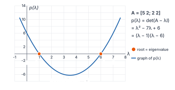
The characteristic polynomial of a square matrix A is p(λ) = det(A − λI). Its roots are the eigenvalues of A, so you find eigenvalues by solving the characteristic equation det(A − λI) = 0. For a 2 × 2 matrix, p(λ) = λ² − (tr A)λ + det A, and some matrices have complex eigenvalues.
Before this lesson: Eigenvalues and Eigenvectors, Determinant of a Matrix and Cofactor Expansion
Why the determinant finds eigenvalues
A number λ is an eigenvalue of A when (A − λI)x = 0 has a nonzero solution. That happens exactly when A − λI is not invertible, which means its determinant is 0 (see the invertible matrix theorem).
So instead of testing one λ at a time, treat λ as a variable. The determinant of A − λI is a polynomial in λ, and its roots are every eigenvalue at once.
The characteristic equation
For an n × n matrix A:
p(\lambda) = \det(A - \lambda I) \qquad \text{eigenvalues: } \det(A - \lambda I) = 0- p(λ) has degree n, so A has n eigenvalues counted with multiplicity, some possibly complex.
- The algebraic multiplicity of an eigenvalue is the number of times it appears as a root of p(λ).
- The sum of the eigenvalues is the trace of A (the sum of the diagonal entries), and their product is det A.
- A real matrix can have complex eigenvalues. They come in conjugate pairs a ± bi.
The 2 × 2 shortcut. For A = \begin{bmatrix} a & b \\ c & d \end{bmatrix}:
\det(A - \lambda I) = (a - \lambda)(d - \lambda) - bc = \lambda^2 - (a + d)\lambda + (ad - bc)
How to find eigenvalues with the characteristic polynomial
- Subtract λ from each diagonal entry to form A − λI.
- Find det(A − λI). For a 3 × 3 matrix, expand along the row or column with the most zeros.
- Set the polynomial equal to 0 and solve. Factor when you can, or use the quadratic formula.
- For each eigenvalue, row reduce A − λI to find its eigenvectors.
- Check: the eigenvalues should add to the trace and multiply to the determinant.
Characteristic polynomial examples
Example 1: Eigenvalues of a 2 × 2 matrix
Find the characteristic polynomial and eigenvalues of A = \begin{bmatrix} 5 & 2 \\ 2 & 2 \end{bmatrix}.
\det(A - \lambda I) = \begin{vmatrix} 5 - \lambda & 2 \\ 2 & 2 - \lambda \end{vmatrix}Subtract λ from each diagonal entry.
= (5 - \lambda)(2 - \lambda) - 2 \cdot 2
Use the 2 × 2 determinant formula.
= 10 - 7\lambda + \lambda^2 - 4
Multiply out the binomials (see multiplying binomials).
= \lambda^2 - 7\lambda + 6
Combine like terms.
(\lambda - 1)(\lambda - 6) = 0
Factor the trinomial (see factoring trinomials).
\lambda = 1 \quad \text{or} \quad \lambda = 6Set each factor equal to 0.
1 + 6 = 7 = 5 + 2,\quad 1 \cdot 6 = 6 = 10 - 4
Check: sum = trace and product = det A.
Answer: p(λ) = λ² − 7λ + 6, and the eigenvalues are 1 and 6.
Example 2: Eigenvalues and eigenvectors
Find the eigenvalues of A = \begin{bmatrix} 3 & 4 \\ -1 & -2 \end{bmatrix} and an eigenvector for each.
\operatorname{tr} A = 3 + (-2) = 1,\quad \det A = -6 - (-4) = -2Find the trace and the determinant.
\lambda^2 - \lambda - 2 = 0
Use the 2 × 2 shortcut.
(\lambda - 2)(\lambda + 1) = 0
Factor.
\lambda = 2 \quad \text{or} \quad \lambda = -1Set each factor equal to 0.
A - 2I = \begin{bmatrix} 1 & 4 \\ -1 & -4 \end{bmatrix} \sim \begin{bmatrix} 1 & 4 \\ 0 & 0 \end{bmatrix}R₂ + R₁ → R₂ (for λ = 2).
x_1 = -4x_2 \;\Rightarrow\; v_1 = \begin{bmatrix} -4 \\ 1 \end{bmatrix}x₂ is free; take x₂ = 1.
A + I = \begin{bmatrix} 4 & 4 \\ -1 & -1 \end{bmatrix} \sim \begin{bmatrix} 4 & 4 \\ 0 & 0 \end{bmatrix}R₂ + ¼R₁ → R₂ (for λ = −1).
x_1 = -x_2 \;\Rightarrow\; v_2 = \begin{bmatrix} -1 \\ 1 \end{bmatrix}x₂ is free; take x₂ = 1.
Av_1 = \begin{bmatrix} -12 + 4 \\ 4 - 2 \end{bmatrix} = \begin{bmatrix} -8 \\ 2 \end{bmatrix} = 2v_1Check v₁.
Av_2 = \begin{bmatrix} -3 + 4 \\ 1 - 2 \end{bmatrix} = \begin{bmatrix} 1 \\ -1 \end{bmatrix} = -1v_2Check v₂.
Answer: λ = 2 with eigenvector (−4, 1), and λ = −1 with eigenvector (−1, 1).
Example 3: A 3 × 3 matrix with a repeated eigenvalue
Find the characteristic polynomial and eigenvalues of A = \begin{bmatrix} 2 & 0 & 0 \\ 1 & 4 & -2 \\ 3 & 1 & 1 \end{bmatrix}.
\det(A - \lambda I) = \begin{vmatrix} 2 - \lambda & 0 & 0 \\ 1 & 4 - \lambda & -2 \\ 3 & 1 & 1 - \lambda \end{vmatrix}Subtract λ from each diagonal entry.
= (2 - \lambda)\begin{vmatrix} 4 - \lambda & -2 \\ 1 & 1 - \lambda \end{vmatrix}Expand along row 1, which has two zeros.
= (2 - \lambda)\big[(4 - \lambda)(1 - \lambda) + 2\big]
2 × 2 determinant: subtract (−2)(1) = −2.
= (2 - \lambda)(\lambda^2 - 5\lambda + 6)
(4 − λ)(1 − λ) = 4 − 5λ + λ², then add 2.
= (2 - \lambda)(\lambda - 2)(\lambda - 3)
Factor the trinomial.
= -(\lambda - 2)^2(\lambda - 3)
Write 2 − λ as −(λ − 2).
2 + 2 + 3 = 7 = 2 + 4 + 1
Check: sum of eigenvalues = trace.
Answer: p(λ) = −(λ − 2)²(λ − 3). The eigenvalues are 2 (algebraic multiplicity 2) and 3.
Example 4: Complex eigenvalues
Find the eigenvalues of A = \begin{bmatrix} 1 & -2 \\ 1 & 3 \end{bmatrix} and an eigenvector for the eigenvalue with positive imaginary part.
\operatorname{tr} A = 4,\quad \det A = 3 - (-2) = 5Find the trace and the determinant.
\lambda^2 - 4\lambda + 5 = 0
Use the 2 × 2 shortcut.
\lambda = \dfrac{4 \pm \sqrt{16 - 20}}{2} = \dfrac{4 \pm \sqrt{-4}}{2}Use the quadratic formula.
= \dfrac{4 \pm 2i}{2} = 2 \pm i√−4 = 2i (see complex numbers), then divide by 2.
A - (2 + i)I = \begin{bmatrix} -1 - i & -2 \\ 1 & 1 - i \end{bmatrix}Subtract 2 + i from each diagonal entry.
x_1 + (1 - i)x_2 = 0
Use row 2. Row 1 is a multiple of it, since A − λI is singular.
x_1 = (-1 + i)x_2 \;\Rightarrow\; v = \begin{bmatrix} -1 + i \\ 1 \end{bmatrix}Take x₂ = 1.
Av = \begin{bmatrix} -1 + i - 2 \\ -1 + i + 3 \end{bmatrix} = \begin{bmatrix} -3 + i \\ 2 + i \end{bmatrix}Check: multiply A by v.
(2 + i)(-1 + i) = -2 + 2i - i + i^2 = -3 + i
The first entry of (2 + i)v matches (see operations with complex numbers).
Answer: λ = 2 ± i. An eigenvector for 2 + i is (−1 + i, 1), and its conjugate (−1 − i, 1) goes with 2 − i.
Example 5: Long-run growth of a beetle population
A beetle population has j juveniles and a adults. Each year, every adult produces 3 juveniles, half the juveniles survive to become adults, and half the adults survive. The next year’s counts are L\begin{bmatrix} j \\ a \end{bmatrix} with L = \begin{bmatrix} 0 & 3 \\ 0.5 & 0.5 \end{bmatrix}. Find the eigenvalues of L, and the eigenvector for the positive one. What do they say about the population in the long run?
\det(L - \lambda I) = (0 - \lambda)(0.5 - \lambda) - 3(0.5)
Use the 2 × 2 determinant formula.
= \lambda^2 - 0.5\lambda - 1.5
Multiply out and simplify.
2\lambda^2 - \lambda - 3 = 0
Multiply both sides by 2 to clear decimals.
(2\lambda - 3)(\lambda + 1) = 0
Factor.
\lambda = 1.5 \quad \text{or} \quad \lambda = -1Set each factor equal to 0.
L - 1.5I = \begin{bmatrix} -1.5 & 3 \\ 0.5 & -1 \end{bmatrix} \sim \begin{bmatrix} -1.5 & 3 \\ 0 & 0 \end{bmatrix}R₂ + ⅓R₁ → R₂.
j = 2a \;\Rightarrow\; v = \begin{bmatrix} 2 \\ 1 \end{bmatrix}Row 1 says −1.5j + 3a = 0; take a = 1.
Lv = \begin{bmatrix} 0 + 3 \\ 1 + 0.5 \end{bmatrix} = \begin{bmatrix} 3 \\ 1.5 \end{bmatrix} = 1.5vCheck.
Answer: the eigenvalues are 1.5 and −1. The larger one in size, 1.5, controls the long run: the population grows by about 50% per year and settles toward 2 juveniles for every adult.
Common mistakes
| Mistake | Example of the error | Fix |
|---|---|---|
| Subtracting λ from every entry | Writing A − λI for [5 2; 2 2] as [5 − λ, 2 − λ; 2 − λ, 2 − λ] | λI has λ only on the diagonal, so only the diagonal entries change. |
| Sign error in the 2 × 2 shortcut | Writing λ² + (tr A)λ + det A | The middle term is −(tr A)λ: p(λ) = λ² − (a + d)λ + (ad − bc). |
| Reading eigenvalues off the diagonal of any matrix | Saying [5 2; 2 2] has eigenvalues 5 and 2 | That shortcut works only for triangular matrices. Here the eigenvalues are 1 and 6. |
| Dropping a repeated root | Listing the eigenvalues in Example 3 as just 2 and 3, then expecting trace 5 | Count multiplicity: 2, 2 and 3 add to 7, the trace. |
| Deciding there are no eigenvalues | Stopping when λ² − 4λ + 5 = 0 has a negative discriminant | The eigenvalues are complex, 2 ± i. Every n × n matrix has n eigenvalues over the complex numbers. |
Related ideas
Eigenspace dimension. An eigenvalue with algebraic multiplicity k has an eigenspace of dimension between 1 and k. When every eigenspace is as large as possible, A can be diagonalized, which the next lesson, Diagonalization, covers.
Other characteristic equations. Linear differential equations and recurrence relations have their own characteristic equations. They come from the same idea: look for solutions that are only scaled by the system.
Practice problems
- Find the characteristic polynomial and eigenvalues of \begin{bmatrix} 4 & 1 \\ 2 & 3 \end{bmatrix}.
- Find the eigenvalues of \begin{bmatrix} 2 & -3 \\ 1 & -2 \end{bmatrix}.
- Find the eigenvalues of \begin{bmatrix} 6 & -1 \\ 2 & 3 \end{bmatrix}.
- Find the eigenvalues of \begin{bmatrix} 1 & 4 \\ 1 & 1 \end{bmatrix} and an eigenvector for each.
- Find the characteristic polynomial of \begin{bmatrix} 3 & 1 \\ 0 & 3 \end{bmatrix} and the algebraic multiplicity of its eigenvalue.
- Find the eigenvalues of the 90° rotation matrix \begin{bmatrix} 0 & -1 \\ 1 & 0 \end{bmatrix}.
- Find the eigenvalues of \begin{bmatrix} 3 & -5 \\ 1 & -1 \end{bmatrix} and an eigenvector for 1 + i.
- Find the eigenvalues of \begin{bmatrix} 1 & 0 & 0 \\ 2 & 4 & 1 \\ -1 & 2 & 3 \end{bmatrix}.
- Check that the eigenvalues in Problem 8 add to the trace and multiply to the determinant.
- Find k so that \begin{bmatrix} 2 & k \\ 3 & 1 \end{bmatrix} has 4 as an eigenvalue. Then find its other eigenvalue.
Show answers
1.
\lambda^2 - 7\lambda + 10 = 0
Shortcut: trace 4 + 3 = 7, determinant 12 − 2 = 10.
(\lambda - 2)(\lambda - 5) = 0
Factor.
Answer: p(λ) = λ² − 7λ + 10; the eigenvalues are 2 and 5.
2.
\lambda^2 - 0\lambda + (-4 + 3) = \lambda^2 - 1
Shortcut: trace 2 − 2 = 0, determinant −4 − (−3) = −1.
(\lambda - 1)(\lambda + 1) = 0
Factor the difference of squares.
Answer: λ = 1 and λ = −1.
3.
\lambda^2 - 9\lambda + 20 = 0
Shortcut: trace 9, determinant 18 − (−2) = 20.
(\lambda - 4)(\lambda - 5) = 0
Factor.
Answer: λ = 4 and λ = 5.
4.
\lambda^2 - 2\lambda - 3 = 0
Shortcut: trace 2, determinant 1 − 4 = −3.
(\lambda - 3)(\lambda + 1) = 0
Factor.
A - 3I = \begin{bmatrix} -2 & 4 \\ 1 & -2 \end{bmatrix} \sim \begin{bmatrix} -2 & 4 \\ 0 & 0 \end{bmatrix}R₂ + ½R₁ → R₂ (for λ = 3). Row 1 gives x₁ = 2x₂.
A + I = \begin{bmatrix} 2 & 4 \\ 1 & 2 \end{bmatrix} \sim \begin{bmatrix} 2 & 4 \\ 0 & 0 \end{bmatrix}R₂ − ½R₁ → R₂ (for λ = −1). Row 1 gives x₁ = −2x₂.
Answer: λ = 3 with eigenvector (2, 1); λ = −1 with eigenvector (−2, 1).
5.
(3 - \lambda)(3 - \lambda) - 1 \cdot 0 = (\lambda - 3)^2
2 × 2 determinant of A − λI.
Answer: p(λ) = (λ − 3)². The only eigenvalue is 3, with algebraic multiplicity 2.
6.
\lambda^2 - 0\lambda + (0 + 1) = \lambda^2 + 1 = 0
Shortcut: trace 0, determinant 0 − (−1) = 1.
\lambda^2 = -1 \;\Rightarrow\; \lambda = \pm i
Subtract 1, then take square roots.
Answer: λ = i and λ = −i. No real vector keeps its direction under a 90° rotation.
7.
\lambda^2 - 2\lambda + 2 = 0
Shortcut: trace 2, determinant −3 − (−5) = 2.
\lambda = \dfrac{2 \pm \sqrt{4 - 8}}{2} = \dfrac{2 \pm 2i}{2} = 1 \pm iQuadratic formula.
x_1 + (-2 - i)x_2 = 0 \;\Rightarrow\; v = \begin{bmatrix} 2 + i \\ 1 \end{bmatrix}Row 2 of A − (1 + i)I is [1, −2 − i]; take x₂ = 1.
Av = \begin{bmatrix} 6 + 3i - 5 \\ 2 + i - 1 \end{bmatrix} = \begin{bmatrix} 1 + 3i \\ 1 + i \end{bmatrix}Check: multiply A by v.
(1 + i)(2 + i) = 2 + i + 2i + i^2 = 1 + 3i
The first entry of (1 + i)v matches.
Answer: λ = 1 ± i, and (2 + i, 1) is an eigenvector for 1 + i.
8.
\det(A - \lambda I) = (1 - \lambda)\begin{vmatrix} 4 - \lambda & 1 \\ 2 & 3 - \lambda \end{vmatrix}Expand along row 1.
= (1 - \lambda)(\lambda^2 - 7\lambda + 10)
(4 − λ)(3 − λ) − 2 = 12 − 7λ + λ² − 2.
= (1 - \lambda)(\lambda - 2)(\lambda - 5)
Factor.
Answer: λ = 1, 2 and 5.
9.
1 + 2 + 5 = 8 = 1 + 4 + 3
Sum of eigenvalues = trace.
1 \cdot 2 \cdot 5 = 10 = 1\,(4 \cdot 3 - 1 \cdot 2)
Product of eigenvalues = det A, found by expanding along row 1.
Answer: both checks pass.
10.
\det(A - 4I) = (-2)(-3) - 3k = 6 - 3k
Subtract 4 from each diagonal entry, then take the determinant.
6 - 3k = 0 \;\Rightarrow\; k = 2
4 is an eigenvalue exactly when this determinant is 0.
4 + \lambda_2 = 2 + 1 \;\Rightarrow\; \lambda_2 = -1
The eigenvalues add to the trace, 3.
Answer: k = 2, and the other eigenvalue is −1. Check: 4 · (−1) = −4 = 2 − 6 = det A.
Characteristic polynomial FAQ
What is the characteristic polynomial of a matrix?
It is p(λ) = det(A − λI), a polynomial of degree n for an n × n matrix. Its roots are the eigenvalues of A.
How do you find the eigenvalues of a 2 × 2 matrix?
Solve λ² − (tr A)λ + det A = 0, where tr A is the sum of the diagonal entries. Factor or use the quadratic formula.
Can a real matrix have complex eigenvalues?
Yes. If the characteristic equation has a negative discriminant, the eigenvalues are complex conjugates a ± bi. Rotation matrices are the classic example.
What is the difference between the characteristic polynomial and the characteristic equation?
The polynomial is det(A − λI). The equation sets it equal to 0, det(A − λI) = 0, and its solutions are the eigenvalues.
Summary
- p(λ) = det(A − λI); its roots are the eigenvalues of A.
- For a 2 × 2 matrix, p(λ) = λ² − (tr A)λ + det A.
- Expand 3 × 3 determinants along a row or column with zeros, and keep the factor (a − λ) intact.
- The eigenvalues add to the trace and multiply to the determinant, counted with multiplicity.
- A negative discriminant gives complex conjugate eigenvalues a ± bi.
Previous lesson: Eigenvalues and Eigenvectors
Next lesson: Diagonalization
Back to the Linear Algebra Index