Diagonalization of a Matrix with Examples

Diagonalization writes a square matrix as A = PDP⁻¹, where D is a diagonal matrix of eigenvalues and the columns of P are matching eigenvectors. An n × n matrix is diagonalizable exactly when it has n linearly independent eigenvectors. Once A is diagonalized, powers are easy: Aᵏ = PDᵏP⁻¹.

Before this lesson: Eigenvalues and Eigenvectors, Characteristic Polynomial and Inverse Matrices

What diagonalization means

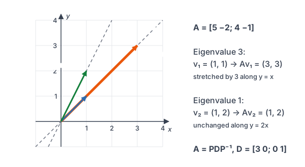
An eigenvector is a direction that A only stretches. If you can find enough eigenvectors to form a basis, then in that basis A does nothing but stretch each coordinate by its eigenvalue. A diagonal matrix does exactly that.

So diagonalization is a change of basis. P⁻¹ converts a vector into eigenvector coordinates, D scales each coordinate, and P converts back. The three steps together do the same thing as A.

Coordinate grid showing the eigenvector directions of the matrix A = [5 −2; 4 −1]. Along the line y = x, the vector v1 = (1, 1) is stretched by 3 to Av1 = (3, 3). Along the line y = 2x, the vector v2 = (1, 2) is unchanged, so Av2 = v2 because its eigenvalue is 1. — Along its eigenvector directions, A = [5 −2; 4 −1] only stretches: by 3 along (1, 1) and by 1 along (1, 2).

The diagonalization theorem

An n × n matrix A is diagonalizable if A = PDP⁻¹ for some invertible matrix P and diagonal matrix D.

A = PDP^{-1} \qquad P = \begin{bmatrix} v_1 & v_2 & \cdots & v_n \end{bmatrix} \qquad D = \begin{bmatrix} \lambda_1 & & \\ & \ddots & \\ & & \lambda_n \end{bmatrix}

A is diagonalizable exactly when it has n linearly independent eigenvectors. They become the columns of P, which is then invertible by the invertible matrix theorem.
Column j of P must be an eigenvector for the eigenvalue in position j of D. Keep the order matched.
If A has n distinct eigenvalues, it is diagonalizable.
With a repeated eigenvalue, A is diagonalizable only if each eigenspace has dimension equal to that eigenvalue’s algebraic multiplicity.
Powers: Aᵏ = PDᵏP⁻¹, and Dᵏ just raises each diagonal entry to the kth power.

Similar matrices. Two matrices A and B are similar if B = P⁻¹AP for some invertible P. Similar matrices have the same characteristic polynomial, so the same eigenvalues, trace and determinant. A diagonalizable matrix is similar to the diagonal matrix D.

How to diagonalize a matrix

Find the eigenvalues by solving det(A − λI) = 0.
For each eigenvalue, find a basis for its eigenspace by row reducing A − λI.
If the eigenspace bases give n vectors in total, A is diagonalizable. If they give fewer, stop: A is not diagonalizable.
Put the eigenvectors in the columns of P and the matching eigenvalues, in the same order, on the diagonal of D.
Check: AP = PD. This check does not need P⁻¹.

Diagonalization examples

Example 1: Diagonalize a 2 × 2 matrix

Diagonalize $A = \begin{bmatrix} 5 & -2 \\ 4 & -1 \end{bmatrix}$ .

\operatorname{tr} A = 5 + (-1) = 4,\quad \det A = -5 - (-8) = 3

Find the trace and the determinant.

\lambda^2 - 4\lambda + 3 = 0

Use the 2 × 2 shortcut λ² − (tr A)λ + det A.

(\lambda - 3)(\lambda - 1) = 0

Factor the trinomial (see factoring trinomials).

\lambda_1 = 3, \quad \lambda_2 = 1

Set each factor equal to 0.

A - 3I = \begin{bmatrix} 2 & -2 \\ 4 & -4 \end{bmatrix} \sim \begin{bmatrix} 2 & -2 \\ 0 & 0 \end{bmatrix}

R₂ − 2R₁ → R₂ (for λ = 3).

x_1 = x_2 \;\Rightarrow\; v_1 = \begin{bmatrix} 1 \\ 1 \end{bmatrix}

x₂ is free; take x₂ = 1.

A - I = \begin{bmatrix} 4 & -2 \\ 4 & -2 \end{bmatrix} \sim \begin{bmatrix} 4 & -2 \\ 0 & 0 \end{bmatrix}

R₂ − R₁ → R₂ (for λ = 1).

x_2 = 2x_1 \;\Rightarrow\; v_2 = \begin{bmatrix} 1 \\ 2 \end{bmatrix}

x₁ is free; take x₁ = 1.

P = \begin{bmatrix} 1 & 1 \\ 1 & 2 \end{bmatrix},\quad D = \begin{bmatrix} 3 & 0 \\ 0 & 1 \end{bmatrix}

Eigenvectors in the columns of P, matching eigenvalues in D.

\det P = 2 - 1 = 1

Find det P (see determinant of a matrix).

P^{-1} = \begin{bmatrix} 2 & -1 \\ -1 & 1 \end{bmatrix}

Swap the diagonal entries, negate the others, divide by det P = 1.

AP = \begin{bmatrix} 5 - 2 & 5 - 4 \\ 4 - 1 & 4 - 2 \end{bmatrix} = \begin{bmatrix} 3 & 1 \\ 3 & 2 \end{bmatrix}

Check: multiply A by P (see matrix multiplication).

PD = \begin{bmatrix} 3 & 1 \\ 3 & 2 \end{bmatrix}

Multiplying by D on the right scales column 1 by 3 and column 2 by 1. AP = PD.

Answer: A = PDP⁻¹ with P = [1 1; 1 2], D = [3 0; 0 1] and P⁻¹ = [2 −1; −1 1].

Example 2: Powers of a matrix

Use the diagonalization in Example 1 to find a formula for Aᵏ, then find A⁴.

A^k = PD^kP^{-1}

The inner P⁻¹P pairs cancel: (PDP⁻¹)(PDP⁻¹) = PD²P⁻¹, and so on.

D^k = \begin{bmatrix} 3^k & 0 \\ 0 & 1 \end{bmatrix}

Raise each diagonal entry to the kth power; 1ᵏ = 1.

PD^k = \begin{bmatrix} 3^k & 1 \\ 3^k & 2 \end{bmatrix}

Scale column 1 of P by 3ᵏ.

A^k = \begin{bmatrix} 3^k & 1 \\ 3^k & 2 \end{bmatrix}\begin{bmatrix} 2 & -1 \\ -1 & 1 \end{bmatrix}

Multiply by P⁻¹ on the right.

= \begin{bmatrix} 2 \cdot 3^k - 1 & -3^k + 1 \\ 2 \cdot 3^k - 2 & -3^k + 2 \end{bmatrix}

Row times column for each entry.

3^4 = 81

Evaluate the power for k = 4 (see exponent rules).

A^4 = \begin{bmatrix} 162 - 1 & -81 + 1 \\ 162 - 2 & -81 + 2 \end{bmatrix}

Substitute 3⁴ = 81, so 2 · 3⁴ = 162.

= \begin{bmatrix} 161 & -80 \\ 160 & -79 \end{bmatrix}

Simplify each entry.

\begin{bmatrix} 2 \cdot 3 - 1 & -3 + 1 \\ 2 \cdot 3 - 2 & -3 + 2 \end{bmatrix} = \begin{bmatrix} 5 & -2 \\ 4 & -1 \end{bmatrix}

Check: k = 1 gives back A.

Answer: Aᵏ = [2 · 3ᵏ − 1, 1 − 3ᵏ; 2 · 3ᵏ − 2, 2 − 3ᵏ], so A⁴ = [161 −80; 160 −79].

Example 3: A repeated eigenvalue that still works

The matrix $A = \begin{bmatrix} 3 & 1 & 1 \\ 1 & 3 & 1 \\ 1 & 1 & 3 \end{bmatrix}$ has eigenvalues 2 (algebraic multiplicity 2) and 5. Diagonalize A.

A - 2I = \begin{bmatrix} 1 & 1 & 1 \\ 1 & 1 & 1 \\ 1 & 1 & 1 \end{bmatrix} \sim \begin{bmatrix} 1 & 1 & 1 \\ 0 & 0 & 0 \\ 1 & 1 & 1 \end{bmatrix}

R₂ − R₁ → R₂ (for λ = 2).

\sim \begin{bmatrix} 1 & 1 & 1 \\ 0 & 0 & 0 \\ 0 & 0 & 0 \end{bmatrix}

R₃ − R₁ → R₃.

x_1 = -x_2 - x_3

Solve row 1 for x₁; x₂ and x₃ are free.

x = x_2\begin{bmatrix} -1 \\ 1 \\ 0 \end{bmatrix} + x_3\begin{bmatrix} -1 \\ 0 \\ 1 \end{bmatrix}

Write the solution in parametric vector form: two eigenvectors for λ = 2.

A - 5I = \begin{bmatrix} -2 & 1 & 1 \\ 1 & -2 & 1 \\ 1 & 1 & -2 \end{bmatrix} \sim \begin{bmatrix} 1 & -2 & 1 \\ -2 & 1 & 1 \\ 1 & 1 & -2 \end{bmatrix}

R₁ ↔ R₂ (for λ = 5).

\sim \begin{bmatrix} 1 & -2 & 1 \\ 0 & -3 & 3 \\ 1 & 1 & -2 \end{bmatrix}

R₂ + 2R₁ → R₂.

\sim \begin{bmatrix} 1 & -2 & 1 \\ 0 & -3 & 3 \\ 0 & 3 & -3 \end{bmatrix}

R₃ − R₁ → R₃.

\sim \begin{bmatrix} 1 & -2 & 1 \\ 0 & -3 & 3 \\ 0 & 0 & 0 \end{bmatrix}

R₃ + R₂ → R₃.

x_2 = x_3

Row 2: −3x₂ + 3x₃ = 0; x₃ is free.

x_1 = 2x_2 - x_3 = x_3

Row 1: x₁ = 2x₂ − x₃, then substitute x₂ = x₃.

v_3 = \begin{bmatrix} 1 \\ 1 \\ 1 \end{bmatrix}

Take x₃ = 1.

P = \begin{bmatrix} -1 & -1 & 1 \\ 1 & 0 & 1 \\ 0 & 1 & 1 \end{bmatrix},\quad D = \begin{bmatrix} 2 & 0 & 0 \\ 0 & 2 & 0 \\ 0 & 0 & 5 \end{bmatrix}

Three eigenvectors in total, so A is diagonalizable.

AP = \begin{bmatrix} -2 & -2 & 5 \\ 2 & 0 & 5 \\ 0 & 2 & 5 \end{bmatrix}

Check: multiply A by P.

PD = \begin{bmatrix} -2 & -2 & 5 \\ 2 & 0 & 5 \\ 0 & 2 & 5 \end{bmatrix}

Scale the columns of P by 2, 2 and 5. AP = PD.

Answer: A = PDP⁻¹ with the P and D above. The eigenvalue 2 is repeated, but its eigenspace has dimension 2, so there are enough eigenvectors.

Example 4: A matrix that is not diagonalizable

Decide whether $A = \begin{bmatrix} 2 & 1 \\ -1 & 4 \end{bmatrix}$ is diagonalizable.

\operatorname{tr} A = 6,\quad \det A = 8 - (-1) = 9

Find the trace and the determinant.

\lambda^2 - 6\lambda + 9 = 0

Use the 2 × 2 shortcut.

(\lambda - 3)^2 = 0

Factor the perfect square trinomial.

\lambda = 3

One eigenvalue, with algebraic multiplicity 2.

A - 3I = \begin{bmatrix} -1 & 1 \\ -1 & 1 \end{bmatrix} \sim \begin{bmatrix} -1 & 1 \\ 0 & 0 \end{bmatrix}

R₂ − R₁ → R₂.

x_1 = x_2 \;\Rightarrow\; v = \begin{bmatrix} 1 \\ 1 \end{bmatrix}

Only one free variable, so the eigenspace has dimension 1.

Answer: A is not diagonalizable. It needs 2 independent eigenvectors, but every eigenvector is a multiple of (1, 1).

Example 5: Bike-share stations in the long run

A bike-share system has two stations. Each day, 10% of the bikes at station A end the day at station B, and 20% of the bikes at B end at A. The rest stay put. The counts after k days are $x_k = M^k x_0$ with $M = \begin{bmatrix} 0.9 & 0.2 \\ 0.1 & 0.8 \end{bmatrix}$ and $x_0 = \begin{bmatrix} 300 \\ 600 \end{bmatrix}$ . Find a formula for xₖ, the counts after 2 days, and the long-run counts.

\operatorname{tr} M = 1.7,\quad \det M = 0.72 - 0.02 = 0.7

Find the trace and the determinant.

\lambda^2 - 1.7\lambda + 0.7 = 0

Use the 2 × 2 shortcut.

(\lambda - 1)(\lambda - 0.7) = 0

Factor: the roots multiply to 0.7 and add to 1.7.

M - I = \begin{bmatrix} -0.1 & 0.2 \\ 0.1 & -0.2 \end{bmatrix} \;\Rightarrow\; v_1 = \begin{bmatrix} 2 \\ 1 \end{bmatrix}

For λ = 1, row 2 says x₁ = 2x₂; take x₂ = 1.

M - 0.7I = \begin{bmatrix} 0.2 & 0.2 \\ 0.1 & 0.1 \end{bmatrix} \;\Rightarrow\; v_2 = \begin{bmatrix} 1 \\ -1 \end{bmatrix}

For λ = 0.7, row 2 says x₁ = −x₂; take x₂ = −1.

c_1\begin{bmatrix} 2 \\ 1 \end{bmatrix} + c_2\begin{bmatrix} 1 \\ -1 \end{bmatrix} = \begin{bmatrix} 300 \\ 600 \end{bmatrix}

Write x₀ in eigenvector coordinates. This is solving Pc = x₀.

3c_1 = 900 \;\Rightarrow\; c_1 = 300

Add the two equations 2c₁ + c₂ = 300 and c₁ − c₂ = 600.

c_2 = 300 - 2(300) = -300

Substitute into the first equation.

x_k = 300(1)^k\begin{bmatrix} 2 \\ 1 \end{bmatrix} - 300(0.7)^k\begin{bmatrix} 1 \\ -1 \end{bmatrix}

M scales each eigenvector by its eigenvalue every day.

= \begin{bmatrix} 600 - 300(0.7)^k \\ 300 + 300(0.7)^k \end{bmatrix}

Combine the vectors.

x_2 = \begin{bmatrix} 600 - 300(0.49) \\ 300 + 300(0.49) \end{bmatrix} = \begin{bmatrix} 453 \\ 447 \end{bmatrix}

For k = 2, (0.7)² = 0.49 and 300(0.49) = 147.

Mx_0 = \begin{bmatrix} 270 + 120 \\ 30 + 480 \end{bmatrix} = \begin{bmatrix} 390 \\ 510 \end{bmatrix}

Check day 1 directly.

Mx_1 = \begin{bmatrix} 351 + 102 \\ 39 + 408 \end{bmatrix} = \begin{bmatrix} 453 \\ 447 \end{bmatrix}

Check day 2 directly. It matches.

(0.7)^k \to 0 \;\Rightarrow\; x_k \to \begin{bmatrix} 600 \\ 300 \end{bmatrix}

As k grows, the λ = 0.7 term dies out.

Answer: xₖ = (600 − 300(0.7)ᵏ, 300 + 300(0.7)ᵏ). After 2 days there are 453 bikes at A and 447 at B. In the long run the counts settle at 600 at A and 300 at B, along the eigenvector for λ = 1.

Common mistakes

Mistake	Example of the error	Fix
Mismatching the order of P and D	Using P = [1 1; 1 2] with D = [1 0; 0 3] in Example 1	Column j of P goes with entry j of D. Swap one if you swap the other.
Writing the product backward	Computing P⁻¹DP instead of PDP⁻¹	A = PDP⁻¹, which also means D = P⁻¹AP.
Thinking a repeated eigenvalue rules out diagonalization	Calling the matrix in Example 3 not diagonalizable because 2 repeats	Check the eigenspace dimension. In Example 3 it is 2, so A is diagonalizable.
Thinking every matrix is diagonalizable	Building P from the single eigenvector (1, 1) twice in Example 4	P must be invertible. Two copies of the same vector are dependent, so this A is not diagonalizable.
Raising each entry of A to a power	Writing A² = [25 4; 16 1] for A = [5 −2; 4 −1]	Only diagonal matrices power entry by entry. Use Aᵏ = PDᵏP⁻¹.

Related ideas

Distinct eigenvalues are enough. Eigenvectors for different eigenvalues are always linearly independent, so n distinct eigenvalues give n independent eigenvectors. The converse fails: Example 3 is diagonalizable with only two distinct eigenvalues.

Symmetric matrices. A real symmetric matrix, like the one in Example 3, is always diagonalizable, and P can be chosen with orthonormal columns. Orthogonal Diagonalization covers this. The next lesson, Orthogonal Sets and Orthonormal Bases, builds the tools.

Where it is used. Diagonalization powers long-run models like Example 5, which are Markov chains in Finite Math, and it decouples systems of linear differential equations in Differential Equations.

Practice problems

Diagonalize $\begin{bmatrix} 4 & 1 \\ 2 & 3 \end{bmatrix}$ .
Diagonalize $\begin{bmatrix} 1 & 2 \\ 2 & 1 \end{bmatrix}$ .
Is $\begin{bmatrix} 5 & 1 \\ 0 & 5 \end{bmatrix}$ diagonalizable?
Is $\begin{bmatrix} 1 & 3 \\ 0 & 2 \end{bmatrix}$ diagonalizable? If so, give P and D.
Find A = PDP⁻¹ for $P = \begin{bmatrix} 1 & 1 \\ 0 & 1 \end{bmatrix}$ and $D = \begin{bmatrix} 2 & 0 \\ 0 & 3 \end{bmatrix}$ .
Use the formula from Example 2 to find A³ for $A = \begin{bmatrix} 5 & -2 \\ 4 & -1 \end{bmatrix}$ .
A 3 × 3 matrix has eigenvalues 1, 4 and 6. Is it diagonalizable? Explain.
The matrix $\begin{bmatrix} 2 & 0 & 0 \\ 0 & 3 & 1 \\ 0 & 0 & 3 \end{bmatrix}$ has eigenvalues 2 and 3. Is it diagonalizable?
Use your answer to Problem 2 to find A⁴ for $A = \begin{bmatrix} 1 & 2 \\ 2 & 1 \end{bmatrix}$ .
Two gyms share 1,000 members. Each month, 20% of gym A’s members switch to gym B and 30% of gym B’s switch to A, so $x_{k+1} = Mx_k$ with $M = \begin{bmatrix} 0.8 & 0.3 \\ 0.2 & 0.7 \end{bmatrix}$ . Starting from $x_0 = \begin{bmatrix} 500 \\ 500 \end{bmatrix}$ , find xₖ and the long-run membership.

Show answers

\lambda^2 - 7\lambda + 10 = 0

Shortcut: trace 4 + 3 = 7, determinant 12 − 2 = 10.

(\lambda - 5)(\lambda - 2) = 0

Factor.

A - 5I = \begin{bmatrix} -1 & 1 \\ 2 & -2 \end{bmatrix} \;\Rightarrow\; v_1 = \begin{bmatrix} 1 \\ 1 \end{bmatrix}

For λ = 5, row 1 says x₁ = x₂.

A - 2I = \begin{bmatrix} 2 & 1 \\ 2 & 1 \end{bmatrix} \;\Rightarrow\; v_2 = \begin{bmatrix} 1 \\ -2 \end{bmatrix}

For λ = 2, row 1 says x₂ = −2x₁.

Answer: P = [1 1; 1 −2], D = [5 0; 0 2]. Check: AP = [5 2; 5 −4] = PD.

\lambda^2 - 2\lambda - 3 = 0

Shortcut: trace 2, determinant 1 − 4 = −3.

(\lambda - 3)(\lambda + 1) = 0

Factor.

A - 3I = \begin{bmatrix} -2 & 2 \\ 2 & -2 \end{bmatrix} \;\Rightarrow\; v_1 = \begin{bmatrix} 1 \\ 1 \end{bmatrix}

For λ = 3, row 1 says x₁ = x₂.

A + I = \begin{bmatrix} 2 & 2 \\ 2 & 2 \end{bmatrix} \;\Rightarrow\; v_2 = \begin{bmatrix} 1 \\ -1 \end{bmatrix}

For λ = −1, row 1 says x₂ = −x₁.

Answer: P = [1 1; 1 −1], D = [3 0; 0 −1]. Check: AP = [3 −1; 3 1] = PD.

(5 - \lambda)^2 = 0 \;\Rightarrow\; \lambda = 5

The matrix is triangular, so the eigenvalues are the diagonal entries.

A - 5I = \begin{bmatrix} 0 & 1 \\ 0 & 0 \end{bmatrix} \;\Rightarrow\; x_2 = 0

Only x₁ is free, so every eigenvector is a multiple of (1, 0).

Answer: no. The eigenvalue 5 has multiplicity 2 but only a 1-dimensional eigenspace.

\lambda_1 = 1, \quad \lambda_2 = 2

Triangular matrix: read the eigenvalues off the diagonal. They are distinct, so A is diagonalizable.

A - I = \begin{bmatrix} 0 & 3 \\ 0 & 1 \end{bmatrix} \;\Rightarrow\; v_1 = \begin{bmatrix} 1 \\ 0 \end{bmatrix}

For λ = 1, the rows say x₂ = 0.

A - 2I = \begin{bmatrix} -1 & 3 \\ 0 & 0 \end{bmatrix} \;\Rightarrow\; v_2 = \begin{bmatrix} 3 \\ 1 \end{bmatrix}

For λ = 2, row 1 says x₁ = 3x₂.

Answer: yes. P = [1 3; 0 1], D = [1 0; 0 2]. Check: AP = [1 6; 0 2] = PD.

P^{-1} = \begin{bmatrix} 1 & -1 \\ 0 & 1 \end{bmatrix}

det P = 1; swap the diagonal entries and negate the others.

PD = \begin{bmatrix} 2 & 3 \\ 0 & 3 \end{bmatrix}

Scale column 1 of P by 2 and column 2 by 3.

PDP^{-1} = \begin{bmatrix} 2 & -2 + 3 \\ 0 & 0 + 3 \end{bmatrix} = \begin{bmatrix} 2 & 1 \\ 0 & 3 \end{bmatrix}

Multiply by P⁻¹ on the right.

Answer: A = [2 1; 0 3].

3^3 = 27

Evaluate the power for k = 3.

A^3 = \begin{bmatrix} 54 - 1 & -27 + 1 \\ 54 - 2 & -27 + 2 \end{bmatrix}

Substitute into Aᵏ = [2 · 3ᵏ − 1, −3ᵏ + 1; 2 · 3ᵏ − 2, −3ᵏ + 2].

= \begin{bmatrix} 53 & -26 \\ 52 & -25 \end{bmatrix}

Simplify each entry.

Answer: A³ = [53 −26; 52 −25].

Answer: yes. Three distinct eigenvalues give three linearly independent eigenvectors, which is enough for a 3 × 3 matrix.

A - 3I = \begin{bmatrix} -1 & 0 & 0 \\ 0 & 0 & 1 \\ 0 & 0 & 0 \end{bmatrix}

For λ = 3, which has algebraic multiplicity 2.

x_1 = 0, \quad x_3 = 0

Rows 1 and 2; only x₂ is free.

Answer: no. The eigenspace for λ = 3 is spanned by (0, 1, 0) alone, so A has only 2 independent eigenvectors, not 3.

D^4 = \begin{bmatrix} 81 & 0 \\ 0 & 1 \end{bmatrix}

3⁴ = 81 and (−1)⁴ = 1.

P^{-1} = \dfrac{1}{-2}\begin{bmatrix} -1 & -1 \\ -1 & 1 \end{bmatrix} = \begin{bmatrix} 0.5 & 0.5 \\ 0.5 & -0.5 \end{bmatrix}

det P = −1 − 1 = −2.

PD^4 = \begin{bmatrix} 81 & 1 \\ 81 & -1 \end{bmatrix}

Scale column 1 of P by 81 and column 2 by 1.

A^4 = \begin{bmatrix} 40.5 + 0.5 & 40.5 - 0.5 \\ 40.5 - 0.5 & 40.5 + 0.5 \end{bmatrix} = \begin{bmatrix} 41 & 40 \\ 40 & 41 \end{bmatrix}

Multiply by P⁻¹ on the right.

Answer: A⁴ = [41 40; 40 41].

10.

(\lambda - 1)(\lambda - 0.5) = 0

Shortcut: trace 1.5, determinant 0.56 − 0.06 = 0.5.

M - I = \begin{bmatrix} -0.2 & 0.3 \\ 0.2 & -0.3 \end{bmatrix} \;\Rightarrow\; v_1 = \begin{bmatrix} 3 \\ 2 \end{bmatrix}

For λ = 1, row 1 says 2x₁ = 3x₂.

M - 0.5I = \begin{bmatrix} 0.3 & 0.3 \\ 0.2 & 0.2 \end{bmatrix} \;\Rightarrow\; v_2 = \begin{bmatrix} 1 \\ -1 \end{bmatrix}

For λ = 0.5, row 1 says x₂ = −x₁.

3c_1 + c_2 = 500, \quad 2c_1 - c_2 = 500

Write x₀ = c₁v₁ + c₂v₂.

c_1 = 200, \quad c_2 = -100

Add the equations: 5c₁ = 1000. Then c₂ = 500 − 600.

x_k = \begin{bmatrix} 600 - 100(0.5)^k \\ 400 + 100(0.5)^k \end{bmatrix}

x_k = 200v₁ − 100(0.5)ᵏv₂.

Answer: xₖ = (600 − 100(0.5)ᵏ, 400 + 100(0.5)ᵏ). In the long run gym A has 600 members and gym B has 400.

Diagonalization FAQ

What does it mean for a matrix to be diagonalizable?

A matrix A is diagonalizable if A = PDP⁻¹ with D diagonal and P invertible. Equivalently, A is similar to a diagonal matrix.

How do you know if a matrix is diagonalizable?

An n × n matrix is diagonalizable exactly when it has n linearly independent eigenvectors. Distinct eigenvalues guarantee this; with a repeated eigenvalue, check that its eigenspace dimension equals its multiplicity.

Why is diagonalization useful?

It turns hard matrix work into work on single numbers. Powers become Aᵏ = PDᵏP⁻¹, which makes long-run models and systems of differential equations much easier to solve.

What are similar matrices?

A and B are similar if B = P⁻¹AP for some invertible P. They describe the same transformation in different bases, so they share eigenvalues, trace and determinant.

Summary

A = PDP⁻¹: eigenvectors in the columns of P, matching eigenvalues on the diagonal of D.
An n × n matrix is diagonalizable exactly when it has n linearly independent eigenvectors.
n distinct eigenvalues guarantee diagonalization; a repeated eigenvalue needs a full-size eigenspace.
Check your work with AP = PD.
Powers: Aᵏ = PDᵏP⁻¹, which shows long-run behavior at a glance.

Previous lesson: Characteristic Polynomial

Next lesson: Orthogonal Sets and Orthonormal Bases

Back to the Linear Algebra Index