
Systems of Differential Equations
A system of differential equations is a set of equations for two or more unknown functions whose derivatives depend on each other. A linear system can be written in matrix form as x′ = Ax. Any higher-order equation can be rewritten as a first-order system by naming each derivative as a new unknown.
Before this lesson: Classifying Differential Equations, Second-Order Homogeneous Linear Equations and Matrix Multiplication
What a system of differential equations is
In one tank, the salt changes at a rate set by that tank alone. Connect two tanks with a pipe, and the salt in the second tank now changes at a rate that depends on the first tank too. The two unknown functions are coupled: you cannot solve for one without knowing something about the other.
A system of differential equations lists one equation for the derivative of each unknown function. A solution is a set of functions, one for each unknown, that makes every equation true at the same time. For two unknowns x(t) and y(t), a solution traces a curve, called a trajectory, in the xy-plane as t increases.
A system is linear when each right side is a sum of the unknowns times coefficients that depend only on t, plus a term that depends only on t. Products like xy, powers like x² and functions like sin x make a system nonlinear.
Systems of differential equations in matrix form
Stack the unknowns into a vector x(t) and their coefficients into a matrix A. A linear system with n unknowns then becomes one vector equation.
\mathbf{x}' = A\mathbf{x} + \mathbf{f}(t), \qquad \mathbf{x} = \begin{bmatrix} x_1 \\ x_2 \\ \vdots \\ x_n \end{bmatrix}Row i of A holds the coefficients of x₁, x₂, …, xₙ in the equation for xᵢ′. The vector f(t) holds the terms with no unknown in them. If f(t) = 0, the system is homogeneous, x′ = Ax. An initial-value problem adds a starting vector x(0).
How to write a higher-order equation as a first-order system
- Solve the equation for its highest derivative, y⁽ⁿ⁾.
- Name new unknowns: x₁ = y, x₂ = y′, …, xₙ = y⁽ⁿ⁻¹⁾.
- Write the chain x₁′ = x₂, x₂′ = x₃, …, up to xₙ₋₁′ = xₙ.
- Write xₙ′ = y⁽ⁿ⁾, using step 1 and replacing y, y′, … by x₁, x₂, ….
- Turn the initial values y(0), y′(0), … into the vector x(0).
This works for every equation, linear or not. It matters because the eigenvalue methods in this unit and numerical solvers such as the Runge-Kutta method are written for first-order systems.
Systems of differential equations examples
Example 1: Matrix form and checking a solution
Write the system x₁′ = x₁ + 2x₂, x₂′ = 3x₁ + 2x₂ in matrix form. Then check that x(t) = (2e^(4t), 3e^(4t)) is a solution.
\mathbf{x}' = \begin{bmatrix} 1 & 2 \\ 3 & 2 \end{bmatrix}\mathbf{x}Row 1 holds the coefficients of x₁′, row 2 those of x₂′.
\mathbf{x}' = \begin{bmatrix} 8e^{4t} \\ 12e^{4t} \end{bmatrix}Differentiate each entry of x(t); the derivative of e^(4t) is 4e^(4t) (see derivatives of exponential functions).
A\mathbf{x} = \begin{bmatrix} 1\cdot 2e^{4t} + 2\cdot 3e^{4t} \\ 3\cdot 2e^{4t} + 2\cdot 3e^{4t} \end{bmatrix}Multiply A by x(t), row by column (see matrix multiplication).
A\mathbf{x} = \begin{bmatrix} 2e^{4t} + 6e^{4t} \\ 6e^{4t} + 6e^{4t} \end{bmatrix}Multiply the constants.
A\mathbf{x} = \begin{bmatrix} 8e^{4t} \\ 12e^{4t} \end{bmatrix}Combine like terms; this matches x′.
Answer: x′ = Ax with A = [1 2; 3 2], and x(t) = (2e^(4t), 3e^(4t)) is a solution. Notice that x(t) = e^(4t)(2, 3), where (2, 3) is an eigenvector of A for the eigenvalue 4. The next lesson builds every solution this way.
Example 2: A second-order equation as a system
Write y″ + 4y′ + 3y = 0 with y(0) = 2 and y′(0) = −4 as a first-order system in matrix form.
y'' = -3y - 4y'
Subtract 3y and 4y′ from both sides to solve for y″.
x_1 = y,\quad x_2 = y'
Name the new unknowns.
x_1' = x_2
The derivative of y is y′.
x_2' = -3x_1 - 4x_2
The derivative of y′ is y″; replace y by x₁ and y′ by x₂.
\mathbf{x}' = \begin{bmatrix} 0 & 1 \\ -3 & -4 \end{bmatrix}\mathbf{x}Write the coefficients as a matrix.
\mathbf{x}(0) = \begin{bmatrix} 2 \\ -4 \end{bmatrix}x₁(0) = y(0) and x₂(0) = y′(0).
Answer: x′ = [0 1; −3 −4]x with x(0) = (2, −4). The matrix has characteristic polynomial λ² + 4λ + 3, the same as the characteristic equation r² + 4r + 3 = 0 of the original equation, so both methods find the same exponents −1 and −3.
Example 3: A third-order equation with forcing
Write y‴ − 2y″ + y′ − 5y = sin t as a first-order system in the form x′ = Ax + f(t).
y''' = 5y - y' + 2y'' + \sin t
Add 5y, subtract y′, add 2y″ and add sin t on both sides to solve for y‴.
x_1 = y,\quad x_2 = y',\quad x_3 = y''
Name three new unknowns.
x_1' = x_2,\quad x_2' = x_3
Write the chain.
x_3' = 5x_1 - x_2 + 2x_3 + \sin t
Replace y, y′ and y″ in the equation for y‴.
\mathbf{x}' = \begin{bmatrix} 0 & 1 & 0 \\ 0 & 0 & 1 \\ 5 & -1 & 2 \end{bmatrix}\mathbf{x} + \begin{bmatrix} 0 \\ 0 \\ \sin t \end{bmatrix}Put the coefficients in A and the term sin t in f(t).
Answer: A = [0 1 0; 0 0 1; 5 −1 2] and f(t) = (0, 0, sin t). The system is linear and nonhomogeneous. A third-order equation always gives three unknowns, and the last row of A holds the coefficients from the solved equation.
Example 4: Two connected tanks (word problem)
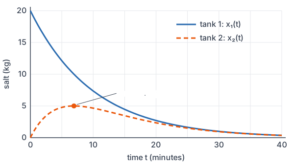
Tank 1 holds 100 L of water with 20 kg of salt dissolved in it. Tank 2 holds 50 L of pure water. Pure water flows into tank 1 at 10 L/min, the mixture flows from tank 1 into tank 2 at 10 L/min, and the mixture leaves tank 2 at 10 L/min. Both tanks stay well mixed. Find the salt amounts x₁(t) and x₂(t) in kilograms, and find when tank 2 holds the most salt.
x_1' = -\dfrac{10}{100}x_1 = -0.1x_1Rate in minus rate out: no salt enters tank 1, and salt leaves at (x₁/100 kg/L)(10 L/min), as in mixing problems.
x_2' = 0.1x_1 - \dfrac{10}{50}x_2 = 0.1x_1 - 0.2x_2Salt from tank 1 enters tank 2, and salt leaves at (x₂/50)(10).
x_1(t) = 20e^{-0.1t}The first equation involves only x₁; it is exponential decay with x₁(0) = 20.
x_2' + 0.2x_2 = 2e^{-0.1t}Substitute x₁ into the second equation and add 0.2x₂ to both sides.
\left(e^{0.2t}x_2\right)' = 2e^{0.1t}Multiply by the integrating factor e^(0.2t) (see first-order linear differential equations).
e^{0.2t}x_2 = 20e^{0.1t} + CIntegrate both sides.
0 = 20 + C \Rightarrow C = -20
Use x₂(0) = 0.
x_2(t) = 20e^{-0.1t} - 20e^{-0.2t}Divide both sides by e^(0.2t).
x_2'(t) = -2e^{-0.1t} + 4e^{-0.2t}Differentiate to find the maximum.
4e^{-0.2t} = 2e^{-0.1t}Set x₂′ = 0 and add 2e^(−0.1t) to both sides.
e^{-0.1t} = \tfrac{1}{2}Divide both sides by 2e^(−0.1t).
t = 10\ln 2 \approx 6.93
Take ln of both sides and divide by −0.1.
x_2 = 20\cdot\tfrac{1}{2} - 20\cdot\tfrac{1}{4}Substitute e^(−0.1t) = 1/2 and e^(−0.2t) = 1/4 into x₂(t).
x_2 = 10 - 5 = 5
Multiply, then subtract.
Answer: x₁(t) = 20e^(−0.1t) and x₂(t) = 20e^(−0.1t) − 20e^(−0.2t) kilograms. Tank 2 holds the most salt, 5 kg, at t = 10 ln 2 ≈ 6.93 minutes. This system was easy because the first equation did not involve x₂; when both equations involve both unknowns, use elimination (Example 5) or eigenvalues.
Example 5: Solving a system by elimination
Solve x′ = x + 2y, y′ = 3x + 2y with x(0) = 4 and y(0) = 1 by turning it into one second-order equation.
y = \tfrac{1}{2}(x' - x)Solve the first equation for y.
y' = \tfrac{1}{2}(x'' - x')Differentiate both sides.
\tfrac{1}{2}(x'' - x') = 3x + 2\cdot\tfrac{1}{2}(x' - x)Substitute y and y′ into the second equation.
x'' - x' = 6x + 2x' - 2x
Multiply both sides by 2.
x'' - 3x' - 4x = 0
Subtract 2x′ and 4x from both sides and combine like terms.
r^2 - 3r - 4 = (r - 4)(r + 1) = 0
Write and factor the characteristic equation (see factoring trinomials).
x = c_1e^{4t} + c_2e^{-t}The roots are 4 and −1 (see second-order homogeneous linear equations).
x' = 4c_1e^{4t} - c_2e^{-t}Differentiate x.
y = \tfrac{1}{2}\left(4c_1e^{4t} - c_2e^{-t} - c_1e^{4t} - c_2e^{-t}\right)Substitute x and x′ into y = (1/2)(x′ − x).
y = \tfrac{3}{2}c_1e^{4t} - c_2e^{-t}Combine like terms and multiply by 1/2.
c_1 + c_2 = 4
Use x(0) = 4.
\tfrac{3}{2}c_1 - c_2 = 1Use y(0) = 1.
\tfrac{5}{2}c_1 = 5 \Rightarrow c_1 = 2Add the two equations (see elimination method) and divide by 5/2.
c_2 = 4 - 2 = 2
Substitute c₁ = 2 into c₁ + c₂ = 4.
x = 2e^{4t} + 2e^{-t},\quad y = 3e^{4t} - 2e^{-t}Substitute c₁ and c₂.
Answer: x(t) = 2e^(4t) + 2e^(−t) and y(t) = 3e^(4t) − 2e^(−t). Check: x′ = 8e^(4t) − 2e^(−t), and x + 2y = 2e^(4t) + 2e^(−t) + 6e^(4t) − 4e^(−t) = 8e^(4t) − 2e^(−t). The e^(4t) part is Example 1’s solution, which is no accident.
Common mistakes
| Mistake | Example of the error | Fix |
|---|---|---|
| Leaving out the chain equations | For y″ = −3y − 4y′, writing only x₂′ = −3x₁ − 4x₂ | Include x₁′ = x₂; a second-order equation gives two equations. |
| Not dividing by the leading coefficient | For 2y″ + 8y′ + 10y = 0, writing x₂′ = −10x₁ − 8x₂ | Solve for y″ first: x₂′ = −5x₁ − 4x₂. |
| Sign errors when solving for the top derivative | y″ − 6y′ + 9y = 0 written as y″ = 6y + 9y′ | Move each term across with the opposite sign: y″ = −9y + 6y′. |
| Putting coefficients in the wrong row | For x′ = 2x − 5y, y′ = x + 3y, writing A = [2 1; −5 3] | Row i lists the coefficients in the equation for the i-th derivative: A = [2 −5; 1 3]. |
| Calling a system with a product linear | x′ = x − xy, y′ = −y + xy treated as x′ = Ax | The term xy makes it nonlinear; it has no matrix form. |
| Mixing up the initial vector | For y(0) = 2, y′(0) = −4, writing x(0) = (−4, 2) | x(0) = (y(0), y′(0)) = (2, −4). |
Related ideas
Nonlinear systems: predator and prey
In the system R′ = 0.4R − 0.02RF, F′ = −0.3F + 0.005RF, R is the number of rabbits and F is the number of foxes. The products RF make it nonlinear, so it has no matrix form. Setting both rates to 0 gives the equilibrium points (0, 0) and (60, 20), where the populations stay constant. Nonlinear Systems and Stability studies how solutions behave near these points.
Solving x′ = Ax with eigenvalues
Elimination works for two unknowns but gets messy for more. The faster method uses the eigenvalues and eigenvectors of A: each eigenvalue λ with eigenvector v gives a solution e^(λt)v, as in Example 1. That is the next lesson, Solving Linear Systems with Eigenvalues.
Second-order models as systems
A spring-mass system my″ + γy′ + ky = 0 becomes a system for position x₁ = y and velocity x₂ = y′. Its trajectory in the x₁x₂-plane is a spiral for damped motion and a closed loop for undamped motion.
Practice problems
- Write the system x′ = 2x − 5y, y′ = x + 3y in matrix form.
- Check that x(t) = (e^(−t), −e^(−t)) is a solution of x₁′ = x₁ + 2x₂, x₂′ = 3x₁ + 2x₂.
- Is x(t) = (e^t, e^t) a solution of the system in Problem 2?
- Write y″ − 6y′ + 9y = 0 with y(0) = 1 and y′(0) = 0 as a first-order system with an initial vector.
- Write 2y″ + 8y′ + 10y = 4 cos 3t in the form x′ = Ax + f(t).
- Write y‴ + 3y″ − y′ + 7y = 0 as a first-order system in matrix form.
- Is the system x′ = t²x + y, y′ = −x + e^t linear? If so, give A(t) and f(t).
- Find the equilibrium points of x′ = x(6 − 2y), y′ = y(x − 3).
- Solve x′ = y, y′ = −4x with x(0) = 1 and y(0) = 0 by elimination.
- Tank 1 holds 400 L with 30 kg of salt, and tank 2 holds 200 L with 10 kg of salt. Pure water flows into tank 1 at 20 L/min, the mixture flows from tank 1 to tank 2 at 20 L/min, and it leaves tank 2 at 20 L/min. Write the system with its initial vector, and find x₁(t).
Show answers
1.
\mathbf{x}' = \begin{bmatrix} 2 & -5 \\ 1 & 3 \end{bmatrix}\mathbf{x}Row 1 holds the coefficients of x′, row 2 those of y′.
Answer: A = [2 −5; 1 3], with x = (x, y)
2.
\mathbf{x}' = \begin{bmatrix} -e^{-t} \\ e^{-t} \end{bmatrix}Differentiate each entry.
A\mathbf{x} = \begin{bmatrix} e^{-t} - 2e^{-t} \\ 3e^{-t} - 2e^{-t} \end{bmatrix}Multiply A = [1 2; 3 2] by x(t).
A\mathbf{x} = \begin{bmatrix} -e^{-t} \\ e^{-t} \end{bmatrix}Combine like terms; this matches x′.
Answer: yes, it is a solution ((1, −1) is an eigenvector for the eigenvalue −1)
3.
\mathbf{x}' = \begin{bmatrix} e^{t} \\ e^{t} \end{bmatrix}Differentiate each entry.
A\mathbf{x} = \begin{bmatrix} e^{t} + 2e^{t} \\ 3e^{t} + 2e^{t} \end{bmatrix} = \begin{bmatrix} 3e^{t} \\ 5e^{t} \end{bmatrix}Multiply A by x(t) and combine like terms.
Answer: no, because Ax = (3e^t, 5e^t) does not equal x′ = (e^t, e^t)
4.
y'' = -9y + 6y'
Subtract 9y and add 6y′ on both sides.
x_1' = x_2,\quad x_2' = -9x_1 + 6x_2
Let x₁ = y and x₂ = y′.
\mathbf{x}' = \begin{bmatrix} 0 & 1 \\ -9 & 6 \end{bmatrix}\mathbf{x},\quad \mathbf{x}(0) = \begin{bmatrix} 1 \\ 0 \end{bmatrix}Write the matrix and the initial vector (y(0), y′(0)).
Answer: x′ = [0 1; −9 6]x, x(0) = (1, 0)
5.
y'' + 4y' + 5y = 2\cos 3t
Divide both sides by 2.
y'' = -5y - 4y' + 2\cos 3t
Subtract 5y and 4y′ from both sides.
x_1' = x_2,\quad x_2' = -5x_1 - 4x_2 + 2\cos 3t
Let x₁ = y and x₂ = y′.
Answer: A = [0 1; −5 −4] and f(t) = (0, 2 cos 3t)
6.
y''' = -7y + y' - 3y''
Subtract 7y, add y′ and subtract 3y″ on both sides.
x_1' = x_2,\quad x_2' = x_3,\quad x_3' = -7x_1 + x_2 - 3x_3
Let x₁ = y, x₂ = y′ and x₃ = y″.
Answer: x′ = [0 1 0; 0 0 1; −7 1 −3]x
7.
\mathbf{x}' = \begin{bmatrix} t^2 & 1 \\ -1 & 0 \end{bmatrix}\mathbf{x} + \begin{bmatrix} 0 \\ e^{t} \end{bmatrix}Each right side is a sum of x and y times functions of t, plus a function of t.
Answer: yes, it is linear (and nonhomogeneous), with A(t) = [t² 1; −1 0] and f(t) = (0, e^t)
8.
x = 0 \text{ or } y = 3Set x′ = 0: a product is 0 when a factor is 0.
y = 0 \text{ or } x = 3Set y′ = 0.
x = 0 \Rightarrow y(-3) = 0 \Rightarrow y = 0
If x = 0, the factor x − 3 is −3, so y must be 0.
y = 3 \Rightarrow 3(x - 3) = 0 \Rightarrow x = 3
If y = 3, then x − 3 must be 0.
Answer: (0, 0) and (3, 3)
9.
x'' = y' = -4x
Differentiate the first equation and substitute the second.
x'' + 4x = 0
Add 4x to both sides.
x = c_1\cos 2t + c_2\sin 2t
The characteristic roots are ±2i (see complex roots of the characteristic equation).
c_1 = 1
Use x(0) = 1.
y = x' = -2c_1\sin 2t + 2c_2\cos 2t
Differentiate x; the first equation says y = x′.
2c_2 = 0 \Rightarrow c_2 = 0
Use y(0) = 0.
Answer: x = cos 2t, y = −2 sin 2t
10.
x_1' = -\dfrac{20}{400}x_1 = -\dfrac{1}{20}x_1Salt leaves tank 1 at (x₁/400)(20) kg/min.
x_2' = \dfrac{1}{20}x_1 - \dfrac{20}{200}x_2 = \dfrac{1}{20}x_1 - \dfrac{1}{10}x_2Salt enters tank 2 from tank 1 and leaves at (x₂/200)(20).
\mathbf{x}(0) = \begin{bmatrix} 30 \\ 10 \end{bmatrix}Initial salt amounts.
x_1(t) = 30e^{-t/20}Exponential decay with x₁(0) = 30.
Answer: x′ = [−1/20 0; 1/20 −1/10]x, x(0) = (30, 10), x₁(t) = 30e^(−t/20)
Systems of differential equations FAQ
What is a system of differential equations?
It is a set of differential equations for two or more unknown functions, where the derivative of each one can depend on the others. A solution is a set of functions that satisfies every equation at once.
How do you convert a second-order differential equation to a system?
Let x₁ = y and x₂ = y′. Then x₁′ = x₂, and x₂′ = y″, which you get by solving the equation for y″ and writing it in terms of x₁ and x₂.
What does x′ = Ax mean?
It is a homogeneous linear system with constant coefficients written in matrix form. The vector x holds the unknown functions, and row i of the matrix A holds the coefficients in the equation for xᵢ′.
Why rewrite a higher-order equation as a first-order system?
First-order systems have one standard form, so one theory and one set of tools covers them all. Eigenvalue methods, phase-plane pictures and numerical solvers such as Runge-Kutta all work on systems.
Summary
- A system of differential equations has two or more unknown functions whose derivatives depend on each other.
- A linear system can be written as x′ = Ax + f(t); it is homogeneous when f(t) = 0.
- To convert an nth-order equation, let x₁ = y, x₂ = y′, …, xₙ = y⁽ⁿ⁻¹⁾ and solve for the highest derivative.
- Some systems can be solved one equation at a time or by elimination; in general, eigenvalues of A give the solutions.
- Products and other nonlinear terms make a system nonlinear; its equilibrium points are where every rate is 0.
Previous lesson: Convolution Theorem
Next lesson: Solving Linear Systems with Eigenvalues
Back to the Differential Equations Index