
Nonlinear Systems and Stability
A nonlinear system x′ = f(x, y), y′ = g(x, y) usually has no formula solution, but near each equilibrium point it acts like a linear system. To study nonlinear systems and stability, find the equilibria, evaluate the Jacobian matrix of partial derivatives there, and classify it with the trace and determinant as a saddle, node or spiral.
Before this lesson: Phase Portraits, Partial Derivatives and Systems of Differential Equations
Why linearization works
Most real models are nonlinear: populations that compete, a swinging pendulum, chemicals that react. Their solutions are hard or impossible to write down. But the behavior near each equilibrium point, where f = 0 and g = 0 at the same time, is usually easy to read.
Close to an equilibrium (x₀, y₀), each function is almost equal to its tangent plane, just as a curve is almost equal to its tangent line in linear approximation. Dropping the small higher-order terms leaves a linear system u′ = Ju, where u = (x − x₀, y − y₀) measures the distance from the equilibrium. This step is called linearization.
The Jacobian matrix
The matrix of the linear system is the Jacobian matrix: the partial derivatives of f in the first row and of g in the second row.
J(x, y) = \begin{bmatrix} f_x & f_y \\ g_x & g_y \end{bmatrix},\qquad \mathbf{u}' = J(x_0, y_0)\,\mathbf{u}Linearization theorem: if no eigenvalue of J(x₀, y₀) has real part 0, the equilibrium has the same type and stability as the linear system. So a linear saddle, node or spiral is also a saddle, node or spiral of the nonlinear system. If J gives a center (pure imaginary eigenvalues) or has a zero eigenvalue, the test is inconclusive: the nonlinear terms decide.
How to classify the equilibria of a nonlinear system
- Solve f(x, y) = 0 and g(x, y) = 0 together to find every equilibrium point.
- Find the four partial derivatives and write J(x, y).
- Evaluate J at each equilibrium.
- Find T and D for each matrix and classify it with the table in phase portraits.
- If the linear result is a center or D = 0, say the test is inconclusive and use another tool, such as a conserved quantity or polar coordinates.
Nonlinear systems and stability examples
Example 1: Two equilibria
Find and classify the equilibrium points of x′ = x − y, y′ = x² − 4.
x - y = 0 \Rightarrow y = x
Set x′ = 0.
x^2 - 4 = 0 \Rightarrow x = \pm 2
Set y′ = 0 and take square roots.
(2, 2),\quad (-2, -2)
Use y = x for each value of x.
J = \begin{bmatrix} 1 & -1 \\ 2x & 0 \end{bmatrix}Take the partial derivatives: f_x = 1, f_y = -1, g_x = 2x, g_y = 0.
J(2, 2) = \begin{bmatrix} 1 & -1 \\ 4 & 0 \end{bmatrix}Substitute x = 2.
T = 1,\quad D = 0 - (-1)(4) = 4
Use T = a + d and D = ad − bc.
T^2 - 4D = 1 - 16 = -15 \lt 0
Complex eigenvalues with positive real part.
J(-2, -2) = \begin{bmatrix} 1 & -1 \\ -4 & 0 \end{bmatrix}Substitute x = −2.
D = 0 - (-1)(-4) = -4 \lt 0
A negative determinant means a saddle.
Answer: (2, 2) is an unstable spiral and (−2, −2) is a saddle. Neither is a center, so the linearization theorem applies to both.
Example 2: A damped pendulum
A damped pendulum satisfies θ″ + 0.5θ′ + sin θ = 0, where θ is the angle from straight down. With ω = θ′, the system is θ′ = ω, ω′ = −sin θ − 0.5ω. Classify the equilibria (0, 0) and (π, 0).
\omega = 0,\quad \sin \theta = 0 \Rightarrow \theta = 0 \text{ or } \piSet both right sides to 0 (other solutions repeat every 2π).
J = \begin{bmatrix} 0 & 1 \\ -\cos \theta & -0.5 \end{bmatrix}The derivative of −sin θ is −cos θ, from derivatives of trig functions.
J(0, 0) = \begin{bmatrix} 0 & 1 \\ -1 & -0.5 \end{bmatrix}Use cos 0 = 1.
T = -0.5,\quad D = 0 - (1)(-1) = 1
Find the trace and determinant.
T^2 - 4D = 0.25 - 4 = -3.75 \lt 0
Complex eigenvalues with negative real part.
J(\pi, 0) = \begin{bmatrix} 0 & 1 \\ 1 & -0.5 \end{bmatrix}Use cos π = −1, so −cos π = 1.
D = 0 - (1)(1) = -1 \lt 0
A negative determinant means a saddle.
Answer: hanging straight down, (0, 0) is a stable spiral: the swings shrink as the pendulum settles. Balanced straight up, (π, 0) is a saddle, so the smallest push makes it fall.
Example 3: Competing species (word problem)
Two species share a food supply. With x and y in hundreds of animals, x′ = x(3 − x − 2y) and y′ = y(2 − x − y). Find and classify every equilibrium, and describe what happens in the long run.
x(3 - x - 2y) = 0 \Rightarrow x = 0 \text{ or } x + 2y = 3Set x′ = 0; a product is 0 when a factor is 0.
y(2 - x - y) = 0 \Rightarrow y = 0 \text{ or } x + y = 2Set y′ = 0 the same way.
(0, 0),\quad (0, 2),\quad (3, 0)
Pair the cases x = 0 or y = 0 with the other equations.
y = 1,\quad x = 1
Subtract x + y = 2 from x + 2y = 3 (elimination method).
J = \begin{bmatrix} 3 - 2x - 2y & -2x \\ -y & 2 - x - 2y \end{bmatrix}Expand to 3x − x² − 2xy and 2y − xy − y², then take partial derivatives.
J(0, 0) = \begin{bmatrix} 3 & 0 \\ 0 & 2 \end{bmatrix}Eigenvalues 3 and 2: unstable node.
J(3, 0) = \begin{bmatrix} -3 & -6 \\ 0 & -1 \end{bmatrix}Triangular, eigenvalues −3 and −1: stable node.
J(0, 2) = \begin{bmatrix} -1 & 0 \\ -2 & -2 \end{bmatrix}Triangular, eigenvalues −1 and −2: stable node.
J(1, 1) = \begin{bmatrix} -1 & -2 \\ -1 & -1 \end{bmatrix}Substitute x = 1 and y = 1.
D = (-1)(-1) - (-2)(-1) = -1 \lt 0
A negative determinant means a saddle.
Answer: (0, 0) is an unstable node, (3, 0) and (0, 2) are stable nodes, and (1, 1) is a saddle. The two species cannot live together: depending on where the populations start, one dies out and the other levels off at its own carrying capacity, as in logistic differential equations.
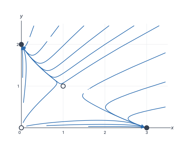
Example 4: Predators and prey
Rabbits x and foxes y follow x′ = x(2 − y) and y′ = y(x − 3). Classify the equilibria, and decide what happens near (3, 2).
x(2 - y) = 0,\quad y(x - 3) = 0
Set both right sides to 0.
(0, 0),\quad (3, 2)
x = 0 forces y = 0; y = 2 forces x = 3.
J = \begin{bmatrix} 2 - y & -x \\ y & x - 3 \end{bmatrix}Partial derivatives of 2x − xy and xy − 3y.
J(0, 0) = \begin{bmatrix} 2 & 0 \\ 0 & -3 \end{bmatrix}Eigenvalues 2 and −3: a saddle.
J(3, 2) = \begin{bmatrix} 0 & -3 \\ 2 & 0 \end{bmatrix}Substitute x = 3 and y = 2.
T = 0,\quad D = 0 - (-3)(2) = 6
The linear system is a center, with λ = ±√6 i.
H = x - 3\ln x + y - 2\ln y
The test is inconclusive, so try a conserved quantity.
\frac{dH}{dt} = \left(1 - \frac{3}{x}\right)x' + \left(1 - \frac{2}{y}\right)y'Use the chain rule.
\frac{dH}{dt} = (x - 3)(2 - y) + (y - 2)(x - 3) = 0Substitute x′ and y′ and simplify.
Answer: (0, 0) is a saddle. At (3, 2) linearization only says center, which is inconclusive. Because H stays constant, each trajectory stays on one closed curve H = constant, so (3, 2) really is a center: the populations cycle forever, with a period near 2π/√6 ≈ 2.57 for small cycles.
Example 5: When linearization fails
Show that the origin of x′ = −y + x(x² + y²), y′ = x + y(x² + y²) linearizes to a center, and then find its true type.
J(0, 0) = \begin{bmatrix} 0 & -1 \\ 1 & 0 \end{bmatrix}The cubic terms have zero partial derivatives at the origin.
T = 0,\quad D = 1
The linear system is a center, so the test is inconclusive.
r^2 = x^2 + y^2 \Rightarrow rr' = xx' + yy'
Use polar coordinates and differentiate r² = x² + y².
xx' + yy' = -xy + x^2r^2 + xy + y^2r^2
Substitute x′ and y′ and multiply.
xx' + yy' = r^2(x^2 + y^2) = r^4
Cancel −xy + xy and factor out r².
r' = r^3
Divide rr′ = r⁴ by r.
Answer: r′ = r³ is positive, so every solution moves away from the origin while it turns: the origin is an unstable spiral. Its linearization is the same center as in Example 4, which shows why a linear center can never decide the question.
Common mistakes
| Mistake | Example of the error | Fix |
|---|---|---|
| Dividing by a variable and losing equilibria | Solving 3 − x − 2y = 0 and dropping x = 0 | Set each factor equal to 0, as in Example 3. |
| Putting partial derivatives in the wrong places | Writing g_x in the top right of J | Row 1 is f_x, f_y; row 2 is g_x, g_y. |
| Evaluating J at the origin for every equilibrium | Using J(0, 0) to classify (1, 1) | Substitute each equilibrium into J separately. |
| Trusting a linear center | Calling the origin of Example 5 a center | A linear center is inconclusive; check with a conserved quantity or r′. |
| Getting the sign of −cos θ wrong | Using −cos π = −1 for the upright pendulum | cos π = −1, so −cos π = 1 and D = −1. |
| Calling a saddle stable because some solutions approach it | Saying (1, 1) in Example 3 is stable | Almost every nearby solution leaves a saddle, so it is unstable. |
Related ideas
Lyapunov functions
The functions H and r² in Examples 4 and 5 are tools of the same kind. If some positive function V decreases along every solution near an equilibrium, the equilibrium is asymptotically stable. Such a V is called a Lyapunov function, and it works even when linearization is inconclusive.
Limit cycles
Some nonlinear systems have an isolated closed trajectory, called a limit cycle, that nearby solutions spiral toward or away from. Linear systems never have one; their closed orbits come in whole families, as in phase portraits of a center.
Practice problems
- Find the equilibrium points of x′ = y − 1, y′ = x² − y.
- Classify the equilibrium (1, 1) of the system in Problem 1.
- Classify the equilibrium (−1, 1) of the system in Problem 1.
- For the undamped pendulum θ′ = ω, ω′ = −sin θ, what does linearization say about (0, 0)?
- For the same pendulum, classify (π, 0).
- For x′ = x(4 − 2x − y), y′ = y(3 − x − y), find the equilibrium with x and y both positive and classify it.
- For the system in Problem 6, classify (2, 0) and (0, 3).
- For x′ = x(1 − 0.5y), y′ = y(0.25x − 1), find the positive equilibrium and say what linearization tells you there.
- Find and classify the equilibria of x′ = y, y′ = −x − y + x².
- For x′ = −y − x³, y′ = x − y³, show that the origin linearizes to a center, and use rr′ to find its true stability.
Show answers
1.
y - 1 = 0 \Rightarrow y = 1
Set x′ = 0.
x^2 - 1 = 0 \Rightarrow x = \pm 1
Substitute y = 1 into x² − y = 0.
Answer: (1, 1) and (−1, 1)
2.
J = \begin{bmatrix} 0 & 1 \\ 2x & -1 \end{bmatrix}Partial derivatives of y − 1 and x² − y.
J(1, 1) = \begin{bmatrix} 0 & 1 \\ 2 & -1 \end{bmatrix},\quad D = 0 - 2 = -2Substitute x = 1; D = (0)(−1) − (1)(2).
Answer: saddle (unstable)
3.
J(-1, 1) = \begin{bmatrix} 0 & 1 \\ -2 & -1 \end{bmatrix}Substitute x = −1.
T = -1,\quad D = 0 - (1)(-2) = 2
Find the trace and determinant.
T^2 - 4D = 1 - 8 = -7 \lt 0
Complex eigenvalues, negative real part.
Answer: stable spiral
4.
J(0, 0) = \begin{bmatrix} 0 & 1 \\ -1 & 0 \end{bmatrix}Use −cos 0 = −1.
T = 0,\quad D = 1
The linear system is a center.
Answer: linearization is inconclusive (a linear center); energy shows it is a true center, since without friction the swings never shrink
5.
J(\pi, 0) = \begin{bmatrix} 0 & 1 \\ 1 & 0 \end{bmatrix}Use −cos π = 1.
D = 0 - 1 = -1 \lt 0
Negative determinant.
Answer: saddle (unstable)
6.
2x + y = 4,\quad x + y = 3
Set the second factors to 0.
x = 1,\quad y = 2
Subtract the second equation from the first, then substitute.
J = \begin{bmatrix} 4 - 4x - y & -x \\ -y & 3 - x - 2y \end{bmatrix}Partial derivatives of 4x − 2x² − xy and 3y − xy − y².
J(1, 2) = \begin{bmatrix} -2 & -1 \\ -2 & -2 \end{bmatrix}Substitute x = 1 and y = 2.
T = -4,\quad D = 4 - 2 = 2
Trace and determinant.
T^2 - 4D = 16 - 8 = 8 \gt 0
Real eigenvalues, both negative.
Answer: (1, 2) is a stable node, so the species can live together
7.
J(2, 0) = \begin{bmatrix} -4 & -2 \\ 0 & 1 \end{bmatrix}Triangular: eigenvalues −4 and 1.
J(0, 3) = \begin{bmatrix} 1 & 0 \\ -3 & -3 \end{bmatrix}Triangular: eigenvalues 1 and −3.
Answer: both are saddles
8.
1 - 0.5y = 0,\quad 0.25x - 1 = 0
Set the second factors to 0.
x = 4,\quad y = 2
Solve each equation.
J(4, 2) = \begin{bmatrix} 0 & -2 \\ 0.5 & 0 \end{bmatrix}J = [1 − 0.5y, −0.5x; 0.25y, 0.25x − 1] at (4, 2).
T = 0,\quad D = 0 - (-2)(0.5) = 1
A linear center.
Answer: (4, 2); linearization is inconclusive (it gives a center)
9.
y = 0,\quad x^2 - x = 0 \Rightarrow x = 0 \text{ or } 1Set y = 0, then factor −x + x² = x(x − 1).
J = \begin{bmatrix} 0 & 1 \\ -1 + 2x & -1 \end{bmatrix}Partial derivatives.
J(0, 0):\ T = -1,\ D = 1,\ T^2 - 4D = -3
Complex eigenvalues, negative real part.
J(1, 0):\ D = 0 - (1)(1) = -1
Negative determinant.
Answer: (0, 0) is a stable spiral and (1, 0) is a saddle
10.
J(0, 0) = \begin{bmatrix} 0 & -1 \\ 1 & 0 \end{bmatrix}The cubic terms drop out: a linear center.
xx' + yy' = -xy - x^4 + xy - y^4
Substitute x′ and y′.
rr' = -(x^4 + y^4) \lt 0
Simplify; it is negative away from the origin.
Answer: r decreases, so the origin is asymptotically stable (a stable spiral), even though the linearization is a center
Nonlinear systems and stability FAQ
What is linearization of a nonlinear system?
It replaces the system near an equilibrium by the linear system u′ = Ju, where J is the Jacobian matrix at that point. Near the equilibrium, the two systems usually have the same type of phase portrait.
What is the Jacobian matrix of a system of differential equations?
For x′ = f(x, y) and y′ = g(x, y), it is the 2 × 2 matrix with f_x and f_y in the first row and g_x and g_y in the second. Its entries depend on the point, so you evaluate it at each equilibrium.
When does linearization fail to classify an equilibrium?
It fails when J has an eigenvalue with real part 0: a linear center or a zero eigenvalue. Then the nonlinear terms decide, and the true point can be a center, a stable spiral or an unstable spiral.
How do you find the equilibrium points of a nonlinear system?
Set every right side equal to 0 and solve the equations together. When an equation factors, set each factor to 0 and pair the cases, so no equilibrium is missed.
Summary
- Equilibria of x′ = f(x, y), y′ = g(x, y) solve f = 0 and g = 0 together.
- The Jacobian matrix J = [f_x f_y; g_x g_y], evaluated at an equilibrium, gives the linearized system u′ = Ju.
- If no eigenvalue of J has real part 0, the equilibrium has the same type and stability as the linear system.
- A linear center (or a zero eigenvalue) is inconclusive; use a conserved quantity, rr′ or a Lyapunov function.
- Competing-species, predator-prey and pendulum models are all studied this way.
Previous lesson: Phase Portraits
Next lesson: Power Series Solutions
Back to the Differential Equations Index